
Relay Based PID Auto-tuning Applied to a Multivariable Level
Control System
Diogo C. Nunes, Jan E. M. G. Pinto, Daniel G. V. Fonseca,
André L. Maitelli and Fábio M. U. Araújo
Federal University of Rio Grande do Norte, Natal, Brazil
Keywords: PID Controllers, Auto-tuning, Multivariable Control, Relay based Tuning.
Abstract: In industrial applications involving control systems, PID controllers are present in the great majority of
them, mostly because of a very simple architecture and easy tuning. For tuning them, the relay method is
also very simple to use and, usually, reach some very satisfactory results, once combined with the
appropriate strategy, like Ziegler-Nichols, Cohen-Coon, CHR, and others. Using this methodology, this
paper presents a relay based PID auto-tuning applied to a multivariable coupled tanks system.
1 INTRODUCTION
Science has traditionally been concerned with
describing nature using mathematical symbols and
equations. More recently, engineers have introduced
(additional) control variables and adjustable
parameters to the mathematical models. Control
engineers want to monitor and control engineering
systems with controllers, which process information
from both desired responses and sensor signals and
affect the behaviour of the system. The field of
control engineers covers the study of dynamical
systems and optimization. If the system is not
performing to expectations, they want to detect this
under-performance from sensors and generate
performance enhancing feedback signals to the
actuators (Tay et. al., 1998).
In the world of control systems, the proportional-
integral-derivative (PID) controller has several
important functions: it provides feedback, it has the
ability to eliminate steady state error through
integral action and it can anticipate the future
through derivative action. PID controllers are
sufficient for many control problems, particularly
when process dynamics are benign and the
performance requirements are modest. In process
control, more than 95% of the control loops are of
PID types, most loops are actually PI control.
(Aström and Hägglund, 1995). In industrial
applications, PID control is a very popular control
strategy due to its simple architecture and easy
tuning. Despite their widespread use and
considerable history, PID tuning is still an active
area of research, both academic and industrial.
(Cong and Liang, 2009).
Aiming for the performance enhancement, some
methods for automatic tuning can be used. By
automatic tuning (or auto-tuning), we mean a
method where the controller is tuned automatically
on demand from a user. Typically, the user will
either push a button or send a command to the
controller. An automatic tuning procedure consists
of three steps: generation of a process disturbance,
evaluation of the disturbance response and
calculation of controller parameters. This is the same
procedure that an experienced operator uses when
tuning a controller manually. The process must be
disturbed in some way in order to determine the
process dynamics. This can be done in many ways,
e.g., by adding steps, pulses, or sinusoidal signals to
the process input. The evaluation of the disturbance
response may include a determination of a process
model or a simple characterization of the response.
(Aström and Hägglund, 1995).
Having well-tuned controllers, with auto-tuning
strategies and tools to track their performance over
time and the ability to retune them, become an item
almost mandatory to maintain processes with high
productivity and low cost, not to mention the quality
of the final product. Researches in the industrial
controllers’ market show that the tuning and/or auto-
tuning function as the most valued by users,
alongside its own PID algorithm and the
741
Nunes D., Pinto J., Fonseca D., Maitelli A. and Araújo F..
Relay Based PID Auto-tuning Applied to a Multivariable Level Control System.
DOI: 10.5220/0005063907410748
In Proceedings of the 11th International Conference on Informatics in Control, Automation and Robotics (ICINCO-2014), pages 741-748
ISBN: 978-989-758-039-0
Copyright
c
2014 SCITEPRESS (Science and Technology Publications, Lda.)

communication protocols (VanDore, 2006).
Among other, the method of step with the relay
feedback (or simply, the relay method) was one of
the first auto-tuning methods to be marketed and
have remained attractive due to its simplicity and
robustness. In addition, many researches have been
conducted to enhance its capability and efficiency.
Furthermore, the PID tuning formulas have been
refined in order to improve the controller
performance for various processes, such as those
with transport delay and oscillations.
Within this scenario, this paper will show an
auto-tuning software used in a multivariable system.
These systems are widely used in the process
industry and academy and many recent papers deal
with them. Saeed et. al. (2010) use a predictive PID
control for a quadruple tank; Tzouanas and
Stevenson (2013) manage the temperature and level
control of a multivariable water tank process;
Ahmed et. al. (2010) bring the discussion of a Fuzzy
model-based predictive control applied to
multivariable level control and De Keyser et. al.
(2013) validate a multivariable relay-based PID
autotuner also using a quadruple tank.
This paper will describe the system used for the
experiments; explain the auto-tuning method build
and evaluate the controller performance before and
after its tuning in order to compare the method
efficacy.
2 COUPLED TANK SYSTEM
For the development of this work, it was used a
coupled tank system simulator, based on a real
(experimental) two-tank system from Quanser
(Figure 1).
Figure 1: Real Coupled Water Tank System from
Quanser.
The two-tank system consists of a pump with a
water basin and two tanks of uniform cross sections.
Such an apparatus forms an autonomous closed and
recirculating system. The two tanks, mounted on the
front plate, are configured such that the flow from
the first (upper) tank can flow into the second
(lower) tank. Flow from the second tank flows into
the main water reservoir. In each one of the two
tanks, liquid is withdrawn from the bottom through
an outflow orifice (i.e. outlet). The outlet pressure is
atmospheric. The water level in each tank is
measured using a pressure-sensitive sensor located
at the bottom of the tank. Additionally, a vertical
scale (in centimeters) is also placed beside each tank
for visual feedback regarding each tank's water
level.
For this experiment, however, it was intended to
use a more complex system. For that, there was the
availability of a simulator with some different
features compared to the Quanser system. It is, for
instance, a five-tank and five-pump system (Figure
2) in which each tank receive liquid from both the
pump and the upper tank (in exception for the first
tank that has only the influence of its pump).
Figure 2: Five-tank system simulator.
The simulator also provides ways for monitoring and
manipulating an experiment, like changing the set-
points, adding disturbances, showing the system’s
process variables (the tanks’ levels, in cetimeters)
and manipulated variables (pumps’ voltages), as
well as others real systems characteristics, like noise
and transport delay.
With this set of features, the simulator is a
PUMP #1
VOLTAGE ON PUMP #3
SET-POINT FOR TANK #1
LEVEL ON
TANK #2
DISTURBANCE
ICINCO2014-11thInternationalConferenceonInformaticsinControl,AutomationandRobotics
742
multivariable coupled tank system that can be used
for various applications. For this paper objective it
will be used for testing and validating tuning
methods in multivariable systems, since it’s dynamic
is based on a real system.
3 PID CONTROLLERS TUNING
STRATEGIES
The main objective of tuning control loop is to
identify the process resulting dynamic to some
control efforts and, based on performance
requirements, define the necessary PID algorithm
dynamics in order to eliminate errors. Those
algorithm dynamics can be defined in many different
forms, depending of the tuning strategy adopted.
Some of these strategies will be shown in the next
sections.
3.1 Ziegler and Nichols
Ziegler and Nichols (1942) developed two empirical
tunings strategies: one based on the system’s step
response in open loop and another based on the
system’s critical gain (
) and critical period (
)
when subjected to a sustained oscillation (such as
the relay experiment) resulting at the equations in
Table 1 for tuning a PID controller.
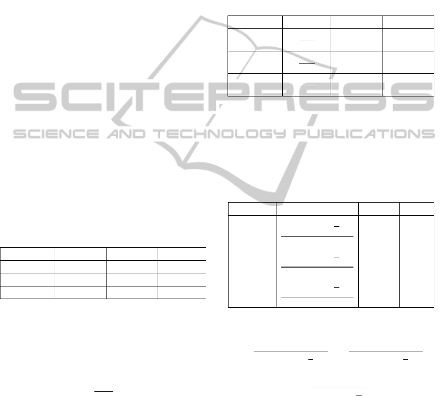
Table 1: Ziegler and Nichols tuning strategy.
Controller
P 0.5
- -
PI 0.45
1.2
⁄
-
PID 0.6
2
⁄
8
⁄
Later, Campos and Teixeira (2006) suggest using
some slack factors or "detuning" to the Ziegler-
Nichols PID tuning strategy due to the uncertainties
of the order of 5% to 20% of the estimated process
dynamics. The usage of these factors result at (1)
and (2).
1.25
(1)
2.5
(2)
3.2 CHR
Developed at the Massachusetts Institute of
Technology, by K. L. Chien, J. A. Hrones and J. B.
Reswick, it was the first tuning strategy to use an
approximate first order model with dead time
representing the behaviour of higher order systems
(Chien et al., 1952). This work was also the pioneer
in the determination of rules for differentiated fit for
servo and regulatory characteristics.
As in Ziegler and Nichols, this strategy also
results in a set of equations (Table 2) to define the
controller parameters, based on the first-order
model’s gain K, dead-time θ and time constant τ.
Table 2: Tuning by CHR strategy.
Controller
P
0.3
- -
PI
0.6
4
-
PID
0.95
2.375 0.421
3.3 Cohen and Coon
The desired result of the Cohen and Coon (1953)
strategy was to tune higher dead time processes, i.e.,
with uncontrollable factor (θ / τ) greater than 0.3.
The tuning equations are shown in Table 3.
Table 3: Cohen and Coon strategy.
Controller
P
1.030.35
- -
PI
1.90.083
-
PID
1.350.25
Where:
0.90.083
1.270.6
,
1.350.25
0.540.6
,
0.5
1.270.6
3.4 IAE, ITAE
A research group from Louisiana State University
(Lopez et al., 1967) developed, in the 60’s, a
methodology for minimizing performance criteria
based on IAE (Integral Absolute Error) and ITAE
(Integral Time Absolute Error). From solving a
RelayBasedPIDAuto-tuningAppliedtoaMultivariableLevelControlSystem
743
problem of multi-objective optimization, they
obtained a set of rules for adjusting the parameters
of the PID controller for different characteristics of a
first order model with dead time, as in Table 4.
Table 4: Tuning strategy based on IAE and ITAE.
Controller
PI - IAE
0.984
.
-
PI - ITAE
0.859
.
-
PID - IAE
1.435
.
PID - ITAE
1.357
.
Where:
0.608
.
,
0.647
.
,
0.878
.
,
0.842
.
,
0.482
.
, 0.381
.
3.5 Internal Model Control (IMC)
The adjustment rules for the IMC strategy are
recommended for the controllability factor (θ / τ) >
0.125 (Rivera et al., 1986). They considered
different process dynamics and obtained PID
controllers for each one depending on the
performance parameter λ. When the process
dynamics can be described by a first-order model
with transport delay, the proposed tuning strategy is
shown in Table 5.
Table 5: IMC strategy.
Controller
PI
2
2
2
-
PID
2
2
2
2
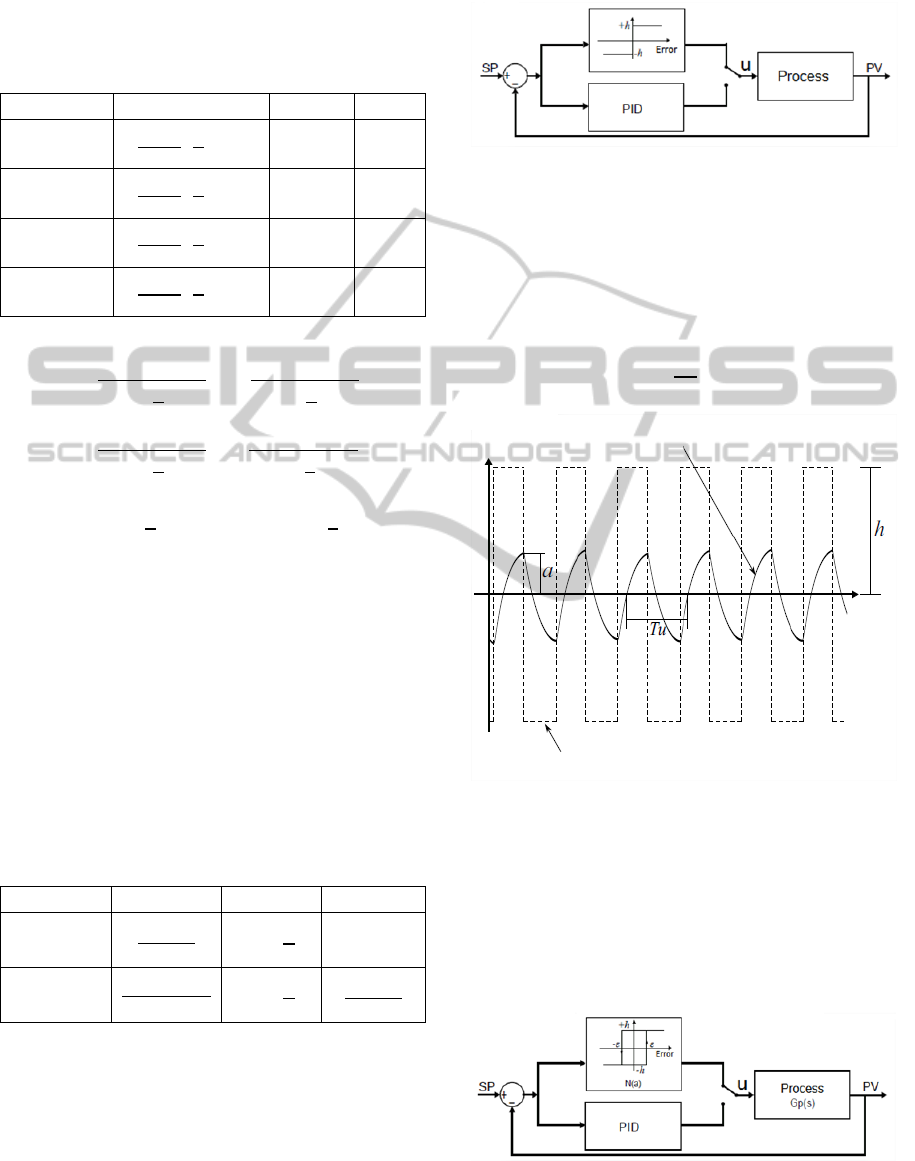
4 RELAY METHOD
The limitations of the Ziegler and Nichols tuning
method led Astrom and Hagglund to propose the use
of a relay in the system to be tuned, creating the
method shown on Figure 3 (Astrom and
Wittenmark, 1988).
Figure 3: Relay method on closed loop.
The purpose of this method is to cause limited and
controlled oscillations in the process and, from its
response (Figure 4), estimate the system’s frequency
response. From the output of amplitude "a" caused
by the relay, the critical gain can be estimated, as in
(3).
4
(3)
Figure 4: System response from the relay method.
The critical period (Tu) is the oscillation period of
the relay itself. With this information on the process
dynamics (Ku and Tu), any tuning strategy (like the
Ziegler and Nichols, for example) can be used to
obtain the values for the PI/PID controller.
Improving the relay to bypass the problem of
unwanted switching caused by noise, Aström and
Figure 5:
Relay with hysteresis
.
S
y
stem response
Rela
y
output
ICINCO2014-11thInternationalConferenceonInformaticsinControl,AutomationandRobotics
744

Hägglund (1984) proposed the use of hysteresis in
the relay (Figure 5).
The relay switch is ruled by the following rule,
where is the hysteresis width:
,
,
,
1
On the developed software, six relay switches
were considered enough to make all necessary
calculations.
In practical applications, the hysteresis should be
selected based on the noise, for example, two times
greater than its amplitude (Hang et al., 2002; Coelho
and dos Santos Coelho, 2004; Campos and Teixeira,
2006) for the establishment of the limit cycle.
The critical frequency (
) is given by (4).
2
(4)
The descriptive function of relay with hysteresis,
designated by is given by (5). This form
comes from approaching the fundamental
component of the Fourier series.
4
∠
(5)
where sin
/.
The system will show a continuous limit cycle
(marginally stable) when the following condition is
satisfied:
1
0
(6)
1
The intersection of the Nyquist plot of
and
–1/ in the complex plane for relay with
hysteresis (Figure 6) results in the process critical
point. The critical gain
, at the critical frequency
, is given by (7).
Figure 6: Nyquist plot.
1
4
(7)
If necessary, it’s also possible, after identifying the
critical point, to define the parameters for a first
order system with transport delay using (8) to
calculate the time constant and (9) to calculate the
transport delay (Cheng, 2006),
1
(8)
(9)
In (8), it is assumed that the process static gain (K)
is known or can be obtained by means of the step
response test (∆ ∆
⁄
). However, even the
relay test data can be used for this purpose, as in
(10) (Hang et al., 2002).
⁄
⁄
(10)
With only the values of
and
obtained from the
relay test, the software can already tune the
controller using the Ziegler-Nichols strategy.
However, with the other parameters (, and ) it
can also use other tables tunings strategies shown on
the section 3 of this paper. Therefore, developed
software is able (with a single relay method
experiment) to determine all these parameters and
generate different tuning parameters so that the user
can compare them in order to choose the most
appropriate one.
5 RESULTS
The tuning software was developed in Java and its
communication with the system variables was via
OPC (OLE for Process Control), which is a widely
used protocol in industry.
Since the system contain five tanks and,
therefore, five control loops, the tuning procedure
need to follow some predefined rules (Campos,
2001):
First, tune the top tank control loop (with all
other in manual operation), since its dynamic
is not affected by the others;
Set the top control loop in automatic operation
(with the calculated tune) and start tuning the
second (from top to bottom) control loop,
whose dynamic is affected only by the already
tuned top tank. The loops below should
RelayBasedPIDAuto-tuningAppliedtoaMultivariableLevelControlSystem
745
remain in manual operation;
Repeat the last rule for the third, fourth and
fifth loop (in this order) always putting the
recently tuned loops in automatic operation;
By the end of the fifth loop, the procedure is
complete.
For each loop tuning process, different tune sets
are proposed by the software, according to the
different strategies used. The user only need to
choose the one that fits the best for each case.
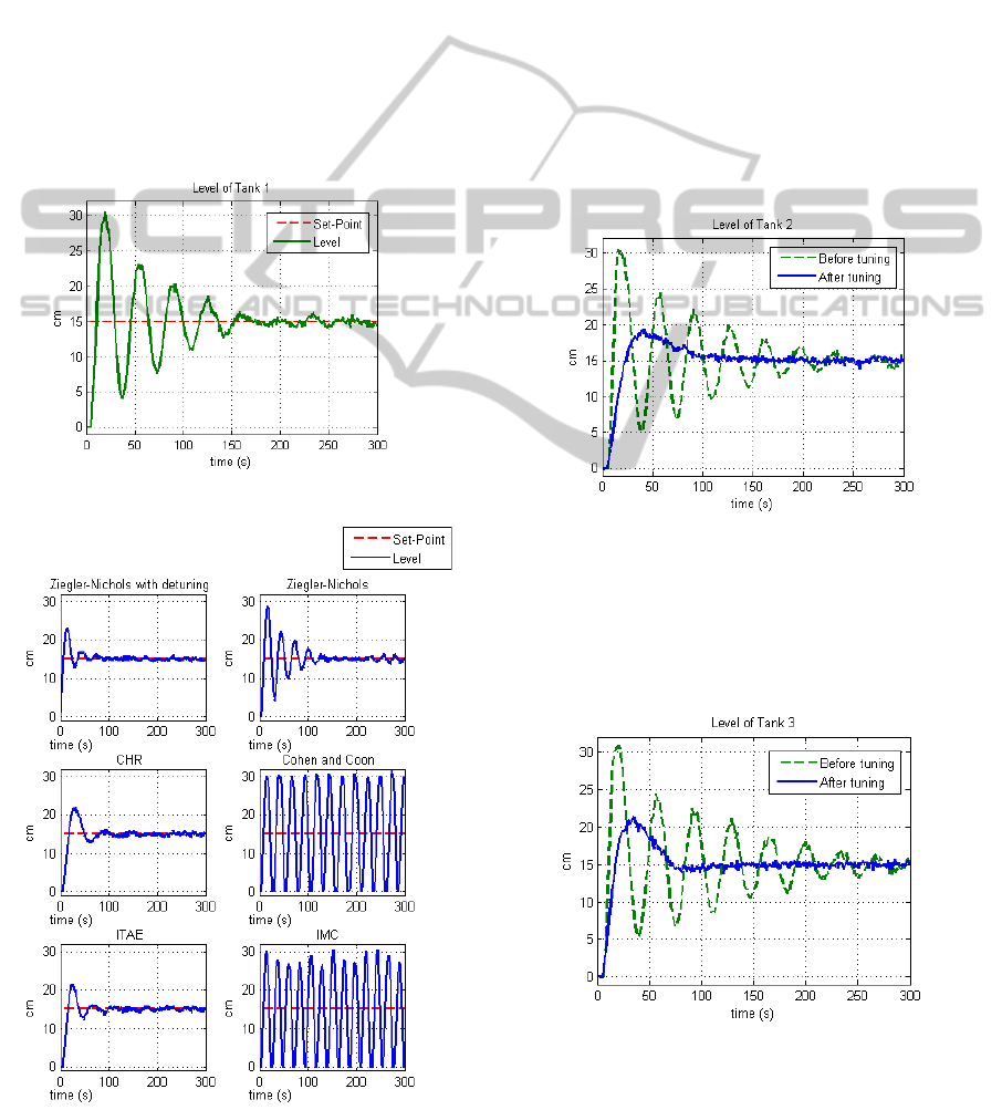
5.1 First Tank Control Loop
Before using the tuning software, it was used a
controller whose parameters were defined by
empiric values, resulting in a poor system response
(Figure 7).
Figure 7: Top control loop before auto-tuning.
Figure 8: Top control loop after auto-tuning.
The tuning software used, then, the relay test to
“study” the system behavior (on a desired operation
point of 15cm, tank’s limits average) and propose
some tuning sets showing several results (Figure 8)
that the user can evaluate. The chosen one for this
loop was the Ziegler-Nichols with ‘detuning’
factors, which resulted in a much better system
response regarding a performance based an minor
overshoot and faster system response. (Figure 8).
5.2 Other Tanks Control Loops
Then, the same procedure was executed for the
second control loop, for which the software showed
some tuning sets and their results when applied to
the system. The chosen set for this loop was also the
one made by the Ziegler-Nichols with ‘detuning’
factors strategy (Figure 9).
Figure 9: Second control loop before and after tuning.
The third control loop, however, was tuned by the
CHR strategy, since it turned out to result in a better
system response (Figure 10). The fourth control loop
was tuned by the Ziegler-Nichols strategy (Figure
11) and the fifth by the ITAE strategy (Figure 12).
Figure 10: Third control loop tuning.
ICINCO2014-11thInternationalConferenceonInformaticsinControl,AutomationandRobotics
746
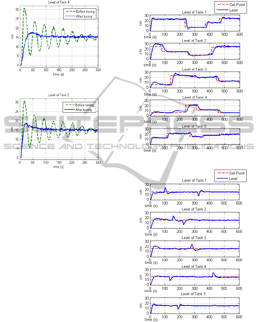
Figure 11: Fourth control loop tuning.
Figure 12: Fifth control loop tuning.
5.3 Other Tests
The tuning results show improvements at the
controllers’ performances, however, those
improvements are shown only at the specific
operation point (15 cm) that was used for the tuning
procedure. In order to really evaluate their
performances, it’s recommended to test the system
with an experiment that takes it to different points,
i.e., a set of different set-points for each control loop
(Figure 13).
An also very important experiment to be made is
a disturbance test, i.e., an experiment that can show
how the system will respond when some disturbance
is applied (Figure 14).
6 CONCLUSIONS
Control engineers, for having to deal with hundreds
of control loops, have the need for methods that
could be easily incorporated in the industry for
tuning and/or auto-tuning of PID controllers. Thus,
the software developed and presented in this paper
for relay based PID tuning fits promisingly, since the
results showed that the procedure introduced by
Figure 13: Test for multiple set-points.
Figure 14: Test for disturbance.
Aström and Hägglund (1984), even after two
decades of evolution of tuning strategies, is still very
satisfactory, with its advantages in simplicity and
RelayBasedPIDAuto-tuningAppliedtoaMultivariableLevelControlSystem
747

robustness. As future prospects, one can think of an
even more automatic tuning method, for example,
using some performances measures like Mean
Squared Error (MSE), Integral Square Error (ISE) or
Integral Time Absolute Error (ITAE). They can help
the software to evaluate the several tuning strategies
results by itself and make a decision of which one is
the best for the system.
ACKNOWLEDGEMENTS
ANP, MCT, FINEP and by Petrobras nancial
support through projects PFRH-220.
REFERENCES
Ahmed, S., Petrov, M. and Ichtev, A. (2010). Fuzzy
Model-Based Predictive Control applied to
multivariable level control of multi tank system. IS
2010 5th IEEE International Conference: 456–461.
Aström, K.J. and Hägglund, T. (1988). Automatic tuning
of simple regulators with specifications on phase and
amplitude margins. Automatica 20(5): 645–651.
Aström, K.J. and Wittenmark, B. (1988). Automatic tuning
of PID Controllers. Instrument Society of America,
Research Triangle Park, North Carolina, USA.
Aström, K.J. and Hägglund, T. (1995). PID Controllers:
Theory, Design and Tuning. Instrument Society of
America, Research Triangle Park, North Carolina,
USA.
Campos, M.C.M.M.D. (2001). Controle Regulatório
Avançado e Sintonia de Controladores PID.
PETROBRAS/CENPES.
Campos, M.C.M.M.D. and Teixeira, H.C.G. (2006).
Controles típicos de equipamentos e processos
industriais. Editora Edgard Blücher, São Paulo, Brazil.
Cheng, C. Y. (2006). Autotuning of PID controllers: a
Relay Feedback Approach, 2nd ed. Springer-Verlag,
London, UK.
Coelho, A. A. R. and dos Santos Coelho, L. (2004).
Identificação de Sistemas Dinâmicos Lineares. Editora
da UFSC, Santa Catarina, Brazil.
Chien, K.L., Hrones, A. and Reswick, J.B. (1952). On the
automatic control of generalized passive systems.
Transactions ASME 74: 175–185.
Cong S. and Liang, Y. (2009). Pid-like neural network
nonlinear adaptive control for uncertain multivariable
motion control systems, IEEE TRANSACTIONS ON
INDUSTRIAL ELECTRONICS 56: 3872-3879.
De Keyser, R., Maxim, A., Copot, C. and Ionescu, C.M.
(2013). Validation of a multivariable relay-based PID
autotuner with specified robustness. ETFA 2013 IEEE
18th Conference: 1–6.
Hang, C.C., Aström, K.J. and Wang, Q.G. (2002). Relay
feedback auto-tuning of process controllers – a
tutorial review, Journal of process control 12(1): 143–
162.
Lopez, A.M., Murrill, P.W. and Smith, C.L. (1967).
Tuning Controllers with Error-Integral Criteria,
Instrumentation Technology 14: 57–62.
Rivera, D.E., Morari, M. and Skogestad, S. (1986).
Internal model control, 4, PID Controller Design
25(1): 252–265.
Saeed, Q., Uddin, V. and Katebi, R. (2010). Multivariable
Predictive PID Control for Quadruple Tank. World
Academy of Science, Engineering and Technology,
International Science Index 43, 4(7): 658–663.
Tay, T.T., Mareels, I. and Moore, J.B. (1998). High
Performance Control. Birkhauser Boston Inc,
Cambridge, MA, USA.
Tzouanas, V. and Stevenson, M. (2013). Temperature and
Level Control of a Multivariable Water Tank Process.
120th ASEE Annual Conference, Atlanta.
VanDore, V. (2006).
Auto-tuning control using Ziegler
Nichols, 9th IEEE/IAS International Conference on
Industry Applications – INDUSCON.
Ziegler, J.G. and Nichols, N.B. (1942). Optimum Settings
for Automatic Control, Transactions ASME 64: 759–
768.
ICINCO2014-11thInternationalConferenceonInformaticsinControl,AutomationandRobotics
748
