
Hierarchical Fuzzy Inductive Reasoning Classifier
Solmaz Bagherpour, Àngela Nebot and Francisco Mugica
Soft Computing Research Group, Technical University of Catalonia, Jordi Girona Salgado 1-3, Barcelona, Spain
Keywords: Fuzzy Inductive Reasoning (FIR), Argument based Machine Learning (ABML), Hierarchical FIR, Zoo
Benchmark.
Abstract: Many of the inductive reasoning algorithms and techniques, including Fuzzy Inductive Reasoning (FIR),
that learn from labelled data don’t provide the possibility of involving domain expert knowledge to induce
rules. In those cases that learning fails, this capability can guide the learning mechanism towards a
hypothesis that seems more promising to a domain expert. One of the main reasons for omitting such
involvement is the difficulty of knowledge acquisition from experts and, also, the difficulty of combining it
with induced hypothesis. One of the successful solutions to such a problem is an alternative approach in
machine learning called Argument Based Machine Learning (ABML) which involves experts in providing
specific explanations in the form of arguments to only specific cases that fail, rather than general knowledge
on all cases. Inspired by this study, the idea of Hierarchical Fuzzy Inductive Reasoning (HFIR) is proposed
in this paper as the first step towards design and development of an Argument Based Fuzzy Inductive
Reasoning method capable of providing domain expert involvement in its induction process. Moreover,
HFIR is able to obtain better classifications results than classical FIR methodology. In this work, the
concept of Hierarchical Fuzzy Inductive Reasoning is introduced and explored by means of the Zoo UCI
benchmark.
1 INTRODUCTION
Uncertainty due to lack of enough information is a
pervasive problem in decision making and
prediction. Nowadays there are many data driven
approaches which has proven good ability in
regression or classification while being able to deal
with uncertainty (Hüllermeier, 2010). However,
almost all of these methods fail when they have to
deal with lack of sufficient information. Lack of
enough information could happen when the
descriptions of available examples in data are not
sufficient to explain the outputs. Almost all of the
data driven approaches including Inductive
Reasoning (IR) and Machine Learning (ML)
methods face similar limitations in such cases
(Wolpert, 1996). Insufficiency of information can
have a more serious impact when the reasoning
system is dealing with many exceptional cases in
data. Complementary approaches can be used in
order to minimize the effect of this phenomenon,
which negatively affects prediction and
classification results.
One of those complementary approaches that can be
applied is argumentation. Medical domain problems,
especially in psychology and psychiatry are one of
the best examples of the explained phenomenon due
to their own uncertain nature (Reichenfeld, 1990).
Patient monitoring and diagnosis applications
empowered by data driven reasoning engines or
automatic classification methods are usually dealing
with both uncertainty and insufficiency of
information (Kononenko, 2001). Uncertainty is due
to their own nature and insufficiency is due to lack
of information on many outlier and exceptional
cases among patients. These exceptional patients are
those patients that in spite of being diagnosed with
the same disorder and in spite of being treated with
the same medications they still respond very
differently comparing to others or most of the
patients. Data driven approaches usually fail to
classify exceptional cases of patients. Such patients
might be exactly those cases which need more
attention and care and they cannot be ignored by the
simple fact of being few. There should be a process
434
Bagherpour S., Nebot À. and Mugica F..
Hierarchical Fuzzy Inductive Reasoning Classifier.
DOI: 10.5220/0005041604340442
In Proceedings of the 4th International Conference on Simulation and Modeling Methodologies, Technologies and Applications (SIMULTECH-2014),
pages 434-442
ISBN: 978-989-758-038-3
Copyright
c
2014 SCITEPRESS (Science and Technology Publications, Lda.)
in handling and remembering them in order to be
able to perform accurate reasoning on new cases.
Fuzzy Inductive Reasoning (FIR) is a data driven
methodology which has proven good ability in
dealing with uncertainty when applied in different
domains including medicine (Nebot and Mugica,
2012). In spite of the good performance of this
method, one of the drawbacks of such modelling
technique in real world applications is when learning
fails because the target hypothesis is very complex,
with many exceptional cases or there is a lack of
sufficient information. One of the burdens of solving
such failures is involvement of domain experts in the
reasoning process because the automatic inductive
reasoning needs guidance to find the acceptable
hypothesis.
Argument Based Machine Learning (ABML) is
one of the latest successful approaches tackling the
same problem in ML methods (Možina et al., 2007;
Mirchevska, 2013). In ABML, some learning
examples are accompanied by arguments that are
expert’s reasons for believing why these examples
are as they are. Thus ABML provides a natural way
of introducing domain-specific prior knowledge in a
way that is different from the traditional, general
background knowledge. The task of ABML is to
find a theory that explains the “argumented”
examples by making reference to the given reasons.
As a refinement to FIR methodology, inspired by
ABML, we believe that an Argument Based Fuzzy
Inductive Reasoning methodology can improve FIR
in dealing with insufficiency of information.
Considering this final goal, the objective of this
article is to introduce a new methodology called
Hierarchical Fuzzy Inductive Reasoning (HFIR)
which is based on FIR and inspired by hierarchical
structure in problem solving as the first step of
developing an Argument Based Fuzzy Inductive
Reasoning methodology. The idea of HFIR is to
design an algorithm that allows the development of a
hierarchy of models that enhances the classification
power of classical FIR methodology. Moreover,
HFIR performs a division of the search space into
several classification subspaces that helps the
identification of rare instances that would probably
need argumentation in order to understand why they
are classified as they are.
The next section introduces the reader to the FIR
methodology. Section 3 describes the HFIR
approach. Section 4 presents the experiments
performed using the Zoo benchmark problem.
Finally the conclusions are outlined.
2 FUZZY INDUCTIVE
REASONING METHODOLOGY
FIR emerged from the General Systems Problem
Solving developed by G. Klir (Klir and Elias, 2002).
It is a data driven methodology based on systems
behaviour rather than on structural knowledge. FIR
reasoning is based on pattern rules synthesized from
the available data. FIR starts with a set of data and
proceeds inductively, learning the behaviour of a
system by observing. FIR can operate on problems
whose structure is not completely known or those
which has high degrees of uncertainty involved in
them (Mugica et al., 2007). In such problems FIR is
able to obtain good qualitative relationships between
the variables that compose the system and to predict
the future behaviour of that system. A FIR model is
a qualitative, non-parametric, shallow model based
on fuzzy logic that runs under the Visual-FIR
platform developed in Matlab (Escobet et al., 2008;
Nebot and Mugica, 2012).
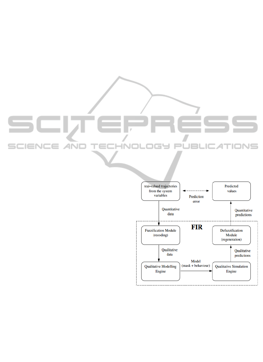
FIR methodology is composed of four basic
modules: fuzzification (fuzzy recoding), qualitative
modelling (fuzzy optimization), qualitative
simulation (fuzzy forecasting), and defuzzification
(fuzzy regeneration), as described in Figure 1.
Figure 1: FIR main processes.
FIR operates on observations of system’s behaviour
of multiple-input single-output. In order to reason
qualitatively about these observed behaviours, real-
valued trajectory behaviour needs to be fuzzified,
i.e. mapped into a set of fuzzy classes. In FIR, the
process of fuzzification is called recoding. In this
process, real-valued data are mapped into qualitative
triples, consisting of a class value (representing a
coarse discretization of the original real-valued
HierarchicalFuzzyInductiveReasoningClassifier
435

variable), a fuzzy membership value (denoting the
level of confidence in the chosen class), and a side
value (telling whether the quantitative value lies to
the left, to the right or at the centre of the
membership function peak). By default in FIR the
data is recoded into an odd number of classes using
the Equal Frequency Partition technique to
determine the landmarks between neighbouring
classes and the fuzzy membership function is a bell-
shaped Gaussian curve that assumes a maximum
value of 1.0 at the centre and a value of 0.5 at each
of the landmarks.
At this point, the continuous trajectory behaviour
recorded from the system has been converted to
episodical behaviour (a qualitative data stream) by
means of the recoding function. In the process of
qualitative modelling, it is desired to discover causal
relations among the variables that make the resulting
state transition matrices as deterministic as possible.
This is accomplished by means of the optimal model
function which is responsible for finding causal,
spatial and temporal relations between variables that
offer the best likelihood for being able to predict the
future system behaviour from its own past.
A FIR model is composed by a set of relevant
variables (feature selection) and a set of input/output
relations called pattern rule base (set of fuzzy rules
that contain the triples mentioned earlier). The
optimality of the selected relevant variables is
evaluated with respect to the maximization of its
forecasting power that is quantified by means of a
quality measure, based mainly on Shannon entropy.
A search in the space of potential sets of relevant
variables must be performed to find the optimal
models for different complexities. The complexity of
a model is defined as the number of relevant
variables selected by this model. Exhaustive and
genetic algorithms are implemented to perform this
search.
Once the most relevant variables are identified,
they are used to derive the set of input/output
relations (or pattern rules) from the training data set.
The FIR qualitative simulation engine is based on
the k-nearest neighbour rule. The forecast of the
output variable is obtained as a weighted average of
the potential conclusions that result from firing the k
rules, whose antecedents best match the actual state.
The defuzzification module, also called fuzzy
regeneration, performs the reverse operation of the
fuzzification module, converting qualitative triples
back to real-valued data. The side value makes it
possible to perform the defuzzification of qualitative
into quantitative values unambiguously and without
information loss.
Due to space limitations it is not possible to go
deeply into FIR methodology. The interested reader
is referred to (Escobet et al., 2008; Nebot and
Mugica, 2012).
3 HIERARCHICAL FUZZY
INDUCTIVE REASONING
METHODOLOGY
One of the basic elements of learning in human
beings is the ability to classify the world at different
granularities and abstraction levels. Classification is
an innate human capability which is related to our
memory as an essential element of human
intelligence. Memory is organized in a way that
interprets present situation based on the information
gained from past situations. These situations and
events are categorized and organized as instances of
classes in our memory. For us even the simplest
tasks require the ability to classify based on our
perception. As mentioned by Estes (1994),
classification is indeed basic to all our intellectual
abilities. Automatic classification is the concept of
interest of this paper because the original FIR offers
scope for improvement to be applied as a classifier
although it is originally designed for regression.
Considering the natural application of multi level
learning by humans, we propose a new method that
modifies original FIR in such a way that
classification is performed at different levels. This
new method results in a Hierarchical Fuzzy
Inductive Reasoning Classifier.
Such type of classifier is interesting for several
reasons. Firstly, in terms of classification accuracy
and, secondly, since the hierarchical FIR can provide
the ability to classify exceptional cases separated
from general classification. These exceptional cases
can be accompanied with arguments of domain
experts as a first step towards an Argument Based
Fuzzy Inductive Reasoning methodology.
FIR defines a single prediction model for each
output. Therefore, if experts want to argument on the
final result of FIR, then their argument would impact
the whole output search space which is not what we
are looking for. A strategy that divides the search
space and learns a FIR model in each of the
subspaces will solve this problem because then the
arguments will impact a specific subspace.
HFIR is designed to be applied in problems with
high degree of uncertainty where few training
examples are available or when there is insufficiency
of information in those examples due to many
SIMULTECH2014-4thInternationalConferenceonSimulationandModelingMethodologies,Technologiesand
Applications
436
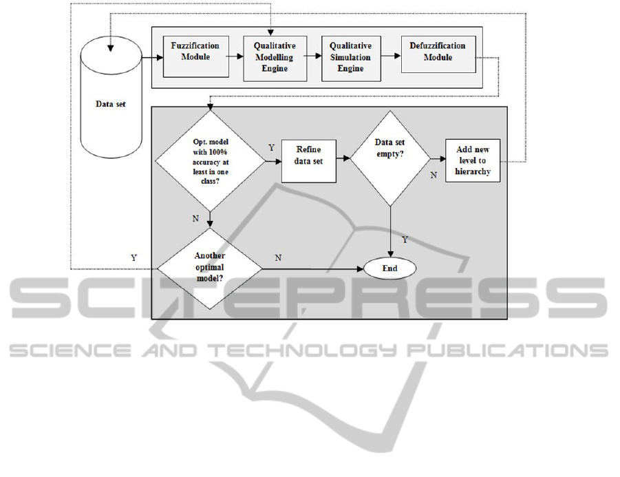
Figure 2: Scheme of HFIR methodology.
exceptional cases. We believe that if we provide a
mechanism for hierarchically solving the
classification problem, then not only the hierarchical
approach will have better classification results
comparing to the classical FIR approach, but also the
hierarchy will deal with a reduced search space.
The reduced search space leads to less general rules,
which, eventually will end up to some exceptional
cases that can’t be classified due to their rarity.
In HFIR, what we mean by Hierarchical
classification is referring to the classification of
multi-class problems through a hierarchical strategy
in obtaining the rules and it shouldn’t be confused
with hierarchical classification problems (Silla and
Freitas, 2011). Hierarchical classification problems
are defined as problems that the classes to be
predicted are organized into a class hierarchy,
typically a tree or a DAG (Directed Acyclic Graph),
due to the hierarchical nature of their data. A
schematic representation of the HFIR methodology
is presented in Figure 2. In such scheme
classification starts at the root with the data set
containing all the available data, then passes through
the four stages of FIR methodology already
explained in Section 2. That is, the data is converted
into fuzzy triples and the optimal qualitative models
for each complexity are identified by FIR
methodology. As explained earlier the qualitative
modelling engine of FIR finds the optimal model of
each complexity from 1 until a parameter value that
specifies the highest complexity that the modeller
wants to study. Then, prediction takes place using
these models which are composed by the selected
relevant variables (feature selection) and the pattern
rule base. The classification errors are calculated by
comparing the real output class values with the
predicted class values. The number of cases that this
comparison does not match corresponds to the
classification error.
At this point, the algorithm selects the optimal
model that has better performance, i.e. the model
with lower complexity that classifies with 100%
accuracy a high (usually the maximum) number of
output classes. Here, a compromise should be taken
between classification performance and complexity
of the model. Once the model is selected, the
algorithm proceeds to the next step that is called
Refine data set. This model represents the first level
of the hierarchy. If none of the models are able to
classify completely one class the algorithm ends.
Now that the first level is shaped, in Refine data
set process the data instances of those classes that
had 100% classification accuracy in the first level
are removed from the whole data set. Then it is
checked if the data set is already empty or not. If
not, it means that there are still remaining classes
which are not classified 100% accurately. Therefore,
a new level is added to the hierarchy by going back
to the initial step but now with the refined data set.
This whole process is repeated until no more
unclassified classes are left or until none of the
optimal models are able to classify correctly another
HierarchicalFuzzyInductiveReasoningClassifier
437

output class. When no more 100% correctly
classified classes can be obtained, the set of
remaining wrongly predicted cases (usually few) are
selected to be argumented by experts.
4 ZOO BENCHMARK
The HFIR methodology described in the previous
section has been use to classify the well known Zoo
benchmark of the UCI machine learning repository
(UCI-ML-R, 2014). Zoo dataset is chosen to carry
our experiments because it has been used in previous
ABML studies and it is understandable and
argumentable by non-experts only by referring to
encyclopaedia. This database contains 101 instances
of animals with 17 Boolean-valued attributes or
variables listed in Table 1. The type variable appears
to be the output variable with the following
meaning: mammal (1), bird (2), reptile (3), fish (4),
amphibian (5), insect (6) and others (7). The class
mammal has 41 instances, the class bird 20, reptile
only 5, the class fish has 13 instances, amphibian has
only 4, insect has 8 instances and others has 10.
Therefore, this dataset is quite unbalanced.
Table 1: Variables involved in the Zoo data set.
Symbol Name Values I/O
A
1
hair binary Input
A
2
feathers binary Input
A
3
egg binary Input
A
4
milk binary Input
A
5
airborne binary Input
A
6
aquatic binary Input
A
7
predator binary Input
A
8
toothed binary Input
A
9
backbone binary Input
A
10
breathes binary Input
A
11
venomous binary Input
A
12
fins binary Input
A
13
legs 0,2,4,5,6,8 Input
A
14
tail binary Input
A
15
domestic binary Input
A
16
cat size binary Input
A
17
type 1,2,3,4,5,6,7 Output
4.1 Regular Experiment
In this first experiment we are considering all of the
attributes available and listed in Table 1. All of the
input variables except legs are discretized into two
classes since they are Boolean attributes. Legs are
discretized into 6 classes, one for each possible
number of legs. The output attribute, type, is
discretized into 7 classes, one for each type of
animal mentioned earlier.
Table 2 shows the results for the first level of
HFIR. In order to analyze better the proposed HFIR
algorithm, the classification results for all the
optimal models considered (from complexity 1 to 8)
are presented in Table 2. Each column represents
one output class, for example column 1 corresponds
to the mammals, column 2 corresponds to birds, and
so on. The fractions under each class column are the
total number of misclassified cases over the total
number of instances of that class. The blank cells
under some classes mean that all of the instances of
that class are correctly classified. Analyzing Table 2
it is clearly seen that none of the optimal models
obtain 100% accuracy on all of the classes. The
optimal model with best classification results is the
model of complexity two (shaded row), considering
that it is the only one that classifies correctly all the
instances of five classes, i.e. 1, 2, 4, 5 and 6, while it
has only two relevant variables that correspond to
milk (A
4
) and legs (A
13
). With this two attributes the
FIR model is able to differentiate between
mammals, birds, fish, amphibian and insects. The
associated rules are R1, R2, R3, R4 and R5
described in Table 5.
Table 2: First level of HFIR for the regular experiment:
Classification results obtained by each optimal model
(from complexity 1 to complexity 8). Last column lists the
relevant variables that compose the model.
1 2 3 4 5 6 7 Variables
41/41
5/5
4/4 7/10 A
13
5/5 3/10 A
4
,A
13
5/5 4/4 3/10 A
4
,A
9
,A
10
5/5 4/4 4/10 A
2
,A
4
,A
9
,A
10
4/4 2/8 A
2
,A
4
,A
6
,A
9
,A
12
4/5 4/4 1/8 2/10 A
2
,A
4
,A
5
,A
9
,A
10
,
A
12
3/5 4/4 2/10 A
1
,A
2
,A
4
,A
7
,A
9
,
A
10
, A
12
3/5 4/4 2/10 A
1
,A
3
,A
7
,A
8
,A
9
,
A
10
,A
12
,A
16
As can be seen from the results, the model of
complexity two is able to classify also 7 instances
out of 10 in class number 7. However, since this
model is not able to classify correctly all the
instances of this class, all the values of class 7 are
kept in the data set and HFIR methodology will try
to find a better model for classes 7 and 3 in the next
level. Therefore, the first level of the HFIR selects
the model of complexity two. At this point, the
algorithm removes all the instances of classes 1, 2,
4, 5 and 6, that have been 100% accurately
classified, from de dataset.
There are still two classes (3 and 7) left to be
modelled, i.e. the data set is not empty, therefore the
SIMULTECH2014-4thInternationalConferenceonSimulationandModelingMethodologies,Technologiesand
Applications
438
process is repeated, as it is depicted in Figure 2. The
results obtained when the process is repeated for the
second time are presented in Table 3.
Here, the model with lowest complexity is the
one that obtains the best classification results among
all (shaded row in Table 3). In this case the
backbone (A
9
) is the variable selected by the
qualitative modelling engine as most relevant
variable. The set of rules derived from model of
complexity one of Table 3 is listed in Table 4. They
are able to classify correctly all the instances of the
classes reptile and others. Since there are no more
classes with unclassified instances, the HFIR
methodology stops here. Therefore, in this
experiment HFIR only needs two levels to classify
correctly the instances of all classes of the animal
type output variable. However, it is interesting to
analyze the results that are obtained by optimal
models of higher complexities.
Table 3: Second level of HFIR for the regular experiment:
Classification results obtained by each optimal model.
Last column lists the relevant variables of each model.
1 2 3 4 5 6 7 Variables
A
9
A
1
,A
9
1/5
A
1
,A
6
,A
9
1/5
A
1
,A
2
,A
6
,A
9
1/5
A
2
,A
4
,A
6
,A
9
,A
12
2/8 A
2
,A
4
,A
5
,A
9
,A
10
,A
12
1/5
A
1
,A
2
,A
4
,A
5
,A
6
,A
9
, A
12
1/5
A
1
,A
2
,A
4
,A
5
,A
6
,A
9
,A
12
,A
16
Table 4: Set of rules of the optimal model of complexity 1.
Rule Class Rule Conditions
R1 3 A
9
= 1 (with backbone)
R2 7 A
9
= 0 (no backbone)
Notice that there are five models that only have one
misclassified instance of class number 3, i.e. the
class reptile. Looking for this misclassified case, we
found that it is the same instance in all of the models
and correspond to a reptile called sea snake. The sea
snake is an air-breathing snake that lives under
water. However we noticed that, in the data, sea
snake is characterized as a non-breathing reptile and
that it does not lay eggs. That is the reason why FIR
Qualitative modelling process does not find that
variables A
3
(eggs) and A
10
(breathes) are relevant in
these five models. It is a confirmed mistake in data
reported by previous studies like ABML (Možina et
al., 2007). The two wrong classified cases in class 6
(insects) are flea and termite which are also both
exceptional because they are the only aquatic insects
among all other insects in this dataset.
With only two hierarchy levels all the output
classes are predicted 100% correctly while in the
first level (which its result is equivalent to flat FIR
classifier) none of the possible complexities
obtained 100% accuracy on all of the classes.
Therefore, it is concluded that HFIR is able to obtain
better classification results than FIR and implies a
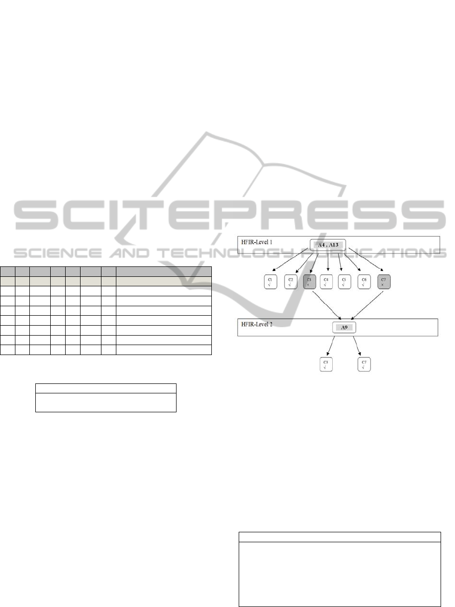
clear improvement. Figure 3 shows schematically
the achieved hierarchy in this experiment. In the first
level, all of the classes with √ sign are those which
all of their instances are correctly classified and
those classes with × sign are the ones that are not
well classified completely. The data of the well
classified classes i.e. C1, C2, C4, C5 and C6, are
removed from the whole dataset and we apply the
HFIR again on the remaining classes shown in gray
in Figure 3, i.e. C3 and C7. In this second level the
model with variable A
9
is chosen as the optimal one
and, with this selection, all of the classes are 100%
classified correctly.
Figure 3: Schematic representation of the HFIR levels for
the Zoo regular experiment.
The classification rules derived from the HFIR
levels of Figure 3 are summarized in Table 5. The
rules are obtained directly from the models in each
level and when descending to the next level, the
rules that describe that level should include the
negation of all the rules of the previous level. This
becomes clear in Table 5.
Table 5: Complete set of rules of the HFIR for the regular
experiment.
Rule Class Rule Conditions
R1 1 A
4
= 1 AND A
13
= 0 OR 2 OR 4
R2 2 A
4
= 0 AND A
13
= 2
R3 4 A
4
= 0 AND A
13
= 0
R4 5 A
4
= 0 AND A
13
= 4
R5 6 A
4
= 0 AND A
13
= 6
R6 7 A
9
= 0 AND NOT(R1,R2,R3,R4,R5)
R7 3 A
9
= 1 AND NOT(R1,R2,R3,R4,R5)
HierarchicalFuzzyInductiveReasoningClassifier
439

The first 5 rules describe the classes well
characterized by the FIR model of the first HFIR
level, i.e. the model that has as relevant variables
milk (A
4
) and legs (A
13
). Rules R6 and R7 are the
rules defined by the optimal model of the second
level of the hierarchy, i.e. the model that has as
relevant variable backbone (A
9
). These two rules
should include the negation of the rules generated in
the previous level, because reaching the second level
means that the first level is not accomplished.
The improvement of using the HFIR proposed
methodology vs. the classical FIR is summarized in
Table 6.
From Table 6 it is clearly seen that the proposed
approach, that performs a hierarchy of models,
outperforms the traditional FIR that is focused on
trying to explain the complete behaviour of a system
by means of a unique model.
Table 6: Percentage of correct classification in all the
output classes when using HFIR and FIR approaches.
1 2 3 4 5 6 7
FIR 100% 100% 0% 100% 100% 100% 30%
HFIR 100% 100% 100% 100% 100% 100% 100%
4.2 Tricky Experiment
In the second experiment with Zoo dataset we want
to force FIR to find relevant attributes alternative to
feathers and milk. Therefore, the attributes A
2
(feathers) and A
4
(milk) are not included in the
dataset of this experiment. We believe that these are
main attributes in classifying the two largest classes
of the dataset, the mammals and the birds. As it can
be seen in the first level of the HFIR in the regular
experiment, milk (A
4
) is selected as relevant variable
in 6 of the 8 FIR optimal models, and feathers (A
2
)
is selected in 4 of the 8 optimal models.
The purpose of this tricky experiment is to
observe the behaviour of HFIR when a constraint is
imposed, i.e. when we remove those variables that
are the most relevant for classifying the largest
classes and the most natural in order to classify
mammals and birds from the human point of view.
We hypothesized that the number of HFIR levels
will grow in this case because each model will
classify correctly a smaller number of animal classes
than in the first experiment.
In order to analyse carefully this issue in this
experiment we proceed in the following way. We
obtain the first level of the hierarchy as in the
regular experiment. From this point, instead of
selecting a specific model from which to proceed to
the second level, we generate the second level
guided by the complexity of each optimal model.
That is, starting from the model of complexity one
obtained in the first level we generate the optimal
model of complexity one of the second level by
removing the instances of the classes 100% correctly
classified in the first level by the model of
complexity one. Then, we generate the optimal
model of complexity two of the second level starting
from the optimal model of complexity 2 obtained in
the first level. We repeat this operation for all the
optimal models of different complexities of level 1.
The results obtained in the first level of the HFIR
are presented in Table 7. From Table 7 it can be seen
that attributes A
1
(hair), A
11
(venomous), A
13
(legs)
and A
15
(domestic) are not relevant for the
classification in the first level. In this case, the
maximum number of classes completely well
classified is 4, but the models that obtain these
results are the ones of higher complexities, i.e. 7 and
8. There are several models of lower complexity that
classify correctly 3 of the 7 output classes.
Therefore, in this case it is difficult to decide which
model to select as the basis to obtain the second
hierarchy level.
Table 7: First level of HFIR for the tricky experiment:
Classification results obtained by each optimal model
(from complexity 1 to complexity 8). Last column lists the
relevant variables that compose the model.
1 2 3 4 5 6 7 Variables
2/41 5/5 4/4
7/10
A
13
41/41 20/2
0
4/5 4/4 8/8 3/10 A
8
,A
10
7/41 5/5 4/4 3/10 A
8
,A
10
,A
14
6/41 5/5
13/1
3
4/4 4/10 A
6
,A
8
,A
9
,
A
12
2/41 4/20 1/5 4/4 2/8 A
3
,A
5
,A
6
,
A
9
,A
12
1/41 4/5 4/4 2/8 A
3
,A
5
,A
8
,
A
9
,A
10
,A
12
4/5 1/4 2/8 A
3
,A
5
,A
8
,
A
9
,A
10
,A
12
, A
14
4/5 3/4 2/10 A
1
,A
3
,A
7
,
A
8
,A
9
,A
10
,
A
12
,A
16
We proceed in the way previously explained to the
next level and we obtain the results shown in Table
8.
The models of higher complexities are able to
classify correctly the rest of the output classes that
where not classified well by the optimal models of
the same complexities in the previous level.
Therefore, if we chose the optimal models of
complexities 7 and 8, only a HFIR of two levels is
needed to classify all the occurrences of the problem
at hand. However, the number of rules derived from
these models is quite large and convoluted.
SIMULTECH2014-4thInternationalConferenceonSimulationandModelingMethodologies,Technologiesand
Applications
440

Table 8: Second level of HFIR for the tricky experiment:
Classification results obtained by each optimal model.
Last column lists the relevant variables of each model.
1 2 3 4 5 6 7 Variables
2/41 5/5 10/10 A
1
7/41
5/5 4/4 8/8 1/10 A
9
,A
15
2/41
4/4
A
3
,A
9
,A
15
2/41 1/5
4/4 2/10 A
1
,A
5
,A
10
,A
14
1/41
5/5 4/4 A
3
,A
8
,A
9
,A
12
,A
16
1/41 1/5 4/4 A
3
,A
8
,A
9
,A
10
,A
12
,
A
16
A
1
,A
3
,A
5
,A
6
,A
9
,
A
10
, A
12
A
1
,A
5
,A
6
,A
8
,A
9
,
A
12
,A
15
,A
16
The models of higher complexities are able to
classify correctly the rest of the output classes that
where not classified well by the optimal models of
the same complexities in the previous level.
Therefore, if we chose the optimal models of
complexities 7 and 8, only a HFIR of two levels is
needed to classify all the occurrences of the problem
at hand. However, the number of rules derived from
these models is quite large and convoluted.
Therefore, it is probably more interesting to obtain a
HFIR with more levels, with less complex optimal
models in each level that allows a better
understanding of the classification rules. This is for
example the case of the optimal models of
complexity 3. In this case a HFIR of three levels is
obtained in order to reach the full classification of
the output variable. This can be seen in the results
obtained at the third level, summarized in Table 9.
Table 9: Third level of HFIR for the tricky experiment.
1 2 3 4 5 6 7 Variables
2/41 5/5
10/10
A
1
2/41
4/4 4/8
A
1
,A
9
A
6
,A
9
,A
16
2/41 1/5
4/4
A
1
,A
6
,A
9
,A
15
1/41
A
3
,A
6
,A
9
,A
10
,
A
15
1/41
A
3
,A
5
,A
6
,A
9
,A
10
A
15
If we continue the experiment to the fourth level, as
shown in Table 10, we reach the point where we
cannot classify completely the remaining classes.
Therefore, if we use complexities 2 or 4, we would
end up to the situation where a specific mammal or a
specific reptile should be argumented by experts.
Table 10: Forth level of HFIR for the tricky experiment.
1 2 3 4 5 6 7 Variables
2/41 5/5 10/10 A
1
1/41
A
3
,A
6
1/5
A
3
,A
6
,A
9,
A
15
The optimal model of complexity 1 is not able to go
further to obtain better classifications. The two
remaining unclassified cases of models of
complexities 2 and 4 are platypus from mammals
and sea snake from reptiles. Platypus among
mammals is exceptional because it is the only
mammal that has hair, eggs, milk, aquatic, predator,
backbone, breathes, four legs, tail and cat size. Sea
snake, as already explained, is an error in the data.
5 CONCLUSIONS
In this paper the Hierarchical Fuzzy Inductive
Reasoning (HFIR) approach for classification is
introduced for the first time. HFIR allows the design
of a hierarchical structure of models that obtains
higher classification accuracy than classical FIR
when used for classification problems and facilitate
the design and development of an Argument Based
FIR methodology. HFIR approach has been
introduced and tested by means of two experiments
over the Zoo UCI benchmark. We are currently
applying the HFIR on more datasets from UCI and,
so far, our preliminary results are promising. In the
near future we plan to test it in real medical data,
specifically in psychology and psychiatry and
compare the results with other classification
methods. Also it would be useful to statistically
prove that the hierarchies won’t increase more than
certain levels.
REFERENCES
Escobet, A., Nebot, A., Cellier, F. E., 2008. Visual-FIR: A
tool for model identification and prediction of
dynamical complex systems, Simulation Modeling
Practice and Theory, vol. 16, nº 1, pp. 76-92.
Estes, W. K., 1994. Classification and Cognition, Oxford
University Press.
Hüllermeier, E., 2010. Uncertainty in Clustering and
Classification. Scalable Uncertainty Management.
Lecture Notes in Computer Science, 6379,pp. 16-19
Klir, G., Elias, D., 2002. Architecture of Systems Problem
Solving, Plenum Press. New York, 2
nd
edition.
Kononenko, I., 2001. Machine learning for medical
diagnosis: history, state of the art and perspective.
Artificial Intelligence in Medicine, 23, pp. 89-109.
Mirchevska, V., 2013. Behavior Modeling by Combining
Machine learning and Domain Knowledge. Ph.D. at
Jozef Stefan International Postgraduate School.
Možina, M., Žabkar, J., Bratko, I., 2007. Argument based
machine learning, Artificial Intelligence, vol. 171, nº
10-15 pp. 922-937.
HierarchicalFuzzyInductiveReasoningClassifier
441

Mugica, F., Nebot, A., Gómez, P., 2007. Dealing with
uncertainty in fuzzy inductive reasoning methodology.
In Proceedings of the Nineteenth Conference on
Uncertainty in Artificial Intelligence (UAI2003),
2012., pp. 922-937.
Nebot, A., Mugica, F., 2012. Fuzzy Inductive Reasoning:
a consolidated approach to data-driven construction of
complex dynamical systems. International Journal of
General Systems, 41(7), pp. 645-665.
Reichenfeld, H.F., 1990. Certainty versus uncertainty in
psychiatric diagnosis. Psychiatr. J. Univ. Ott., 15(4),
pp. 189-93.
Silla, N., Freitas, A. A., 2011. A Survey of Hierarchical
Classification Across Different Application Domains,
Data Mining and Knowledge Discovery, vol. 22, nº 1-
2, pp. 31-72.
UCI Machine Learning Repository, 2014.
http://archive.ics.uci.edu/ml/
Wolpert, D., 1996. The lack of a priori distinctions
between learning algorithms. Neural Computation, 8,
pp. 1341–1390.
SIMULTECH2014-4thInternationalConferenceonSimulationandModelingMethodologies,Technologiesand
Applications
442
