Model Identiﬁcation for Photovoltaic Panels Using Neural Networks

Antonino Laudani, Gabriele Maria Lozito, Martina Radicioni, Francesco Riganti Fulginei

and Alessandro Salvini

Department of Engineering, Roma Tre University, Via Vito Volterra 62/b, Rome, Italy

Keywords:

Neural Networks, Fully Connected Cascade, Photovoltaic Panels, One-Diode Model.

Abstract:

The present work documents the study on the usage of Neural Networks to compute the parameters used in

solar panel modelling. The approach followed starts from a dataset obtained by a process of model identiﬁ-

cation via numerical solution of nonlinear equations. After a preliminary analysis pointing out the intrinsic

difﬁculty in the classic identiﬁcation of the parameters via NN, by taking advantage of closed form relations, a

hybrid neural system, composed by neural network based identiﬁers and explicit equations, was implemented.

The generalization capabilities of the neural identiﬁer were investigated, showing the effectiveness of this

approach.

1 INTRODUCTION

The solar energy power industry requires the use of

suitable photovoltaic (PV) model for the evaluation

of the performance of power plants. Among the

available models for electrical representation of a PV

panel, the ﬁve-parameter one, also known as ”‘one-

diode model”’, is the widest adopted and is gener-

ally recognized as reference design tool (Blair et al.,

2010). This model describes the electrical relation be-

tween current and voltage for a PV module (or an ar-

ray of modules), and may be identiﬁed either by em-

ploying few experimental data, or by solving a system

of ﬁve non-linear equations, starting from data pro-

vided by manufacturers in datasheets. In both cases,

the identiﬁcation problem is really a complicated task,

which must be resolved numerically by means of op-

timization/inverse problems solving techniques. In-

deed, two main issues characterize the model and

must be addressed: the transcendental nature of the

equations, which leads to the impossibility to solve

the problem analytically, and the lack of sufﬁcient

informations to take effective initial guess values to

be used in the selected optimization/inverse problem

technique. For these reasons, almost any possible

optimization technique has been adopted in litera-

ture: simulated annealing (El-Naggar et al., 2012),

genetic algorithm (Zagrouba et al., 2010), differen-

tial evolution (Ishaque and Salam, 2011; Jiang et al.,

2013), evolutionary algorithm (Siddiqui and Abido,

2013), artiﬁcial bee swarm optimization (Askarzadeh

and Rezazadeh, 2013), bacterial foraging algorithm

(Rajasekar et al., 2013), semi-analytical/deterministic

approach and so on. All these techniques, although

effective, make the constrained optimization problem

with ﬁve unknowns rather long and complex to solve

without strong computational capabilities. This short-

coming of the model was addressed in (Laudani et al.,

2013), where the authors deduced that the model

could be reduced, by following algebraic manipula-

tion, to a two only independent parameters model, be-

ing three of the original parameters dependent on the

other two. The resulting model must be still identiﬁed

by numerical means, but now using much less com-

plex methods (deterministic algorithms) such as New-

ton method or steepest descent gradient. In fact, it

has been observed that the two-parameter problem is

usually convex, also in the case of experimental data

(Laudani et al., 2014a). However, regardless of the

used model, the PV parameter identiﬁcation requires

a complex software architecture. The ﬁve-parameter

model needs a high exploration algorithm to isolate

candidate solutions, that are later reﬁned by a local

search algorithm, to discern local minima from global

optimum. The two-parameter reduced form model,

even if convex, still requires a local non-linear opti-

mization algorithm to be efﬁciently identiﬁed (Lau-

dani et al., 2014b): this is a serious drawback, which

does not allow an easy implementation of a generic

solver for the problem outside a suitable computing

environment, such as Matlab. This is a serious limi-

tation, since it does not allow the integration of these

130

Laudani A., Lozito G., Radicioni M., Riganti Fulginei F. and Salvini A..

Model Identiﬁcation for Photovoltaic Panels Using Neural Networks.

DOI: 10.5220/0005039201300137

In Proceedings of the International Conference on Neural Computation Theory and Applications (NCTA-2014), pages 130-137

ISBN: 978-989-758-054-3

 2014 SCITEPRESS (Science and Technology Publications, Lda.)

identiﬁcation algorithms in low cost embedded sys-

tem, based on microncontroller architecture, for the

monitoring and the management of PV plants (Car-

rasco et al., 2013). On the other hand, although many

artiﬁcial intelligence methods have been used for this

problem, the Neural Networks (NNs) were used only

to interpolate experimental data, rather than extract

the ﬁve parameter model. In the PV ﬁeld, NNs are

frequently used for MPPT (Maximum Power Point

Tracking) algorithms (Liu et al., 2013), solar irra-

diance (Mancilla-David et al., 2014) estimation and

forecasting (a review on the subject was published by

(Yadav and Chandel, 2014)). Nevertheless, at the au-

thors knowledge, in literature the neural approach did

not lead to effective results in the PV ﬁve parame-

ter model extraction yet. This probably is due to a

twofold problem: i) the need of a meaningful dataset

for the training of the NN (thanks to which the NN

should be able to learn how to solve the respective

non-linear system of equations) which involves solv-

ing the inverse problem for a high number of differ-

ent panels; ii) the difﬁculties in the identiﬁcation of

one of the parameters (R

), which makes ineffective

the neural approach. On the other hand, Neural Net-

works (NN) are often used in literature to solve efﬁ-

ciently mathematical problems (Capizzi et al., 2004;

Xu et al., 2012) involving solution of complex math-

ematical expression. This paper is aimed at showing

the results obtained by the developed neural network

in the solution of the identiﬁcation problem for the

ﬁve parameter model starting from datasheet informa-

tion, thanks to the synergy between neural approach

and reduced forms.

2 THE FIVE-PARAMETER

MODEL AND ITS REDUCTION

TO TWO PARAMETERS

The ﬁve parameter model is based on the circuit rep-

resentation of a PV module by the means of an in-

dependent current source, an anti-parallel diode and

two output resistances, one in parallel with the diode

and one in series with the output branch (see ﬁg. 1).

The current-voltage relation expressed by the model

is shown in 1.

I = I

Irr

− I



(

V+IR

)

nkT



− 1

−

V + IR

(1)

This equation can represent a PV module composed

by an arbitrary number N

of cells in series. The pa-

rameters of equation (1) are the ideality factor n, the

shunt resistance R

, the series resistance R

, the sat-

uration reversal current of the diode I

and the irra-

diation current I

Irr

. The other physical quantities in-

volved are: the electron charge q (q = 1.602× 10

−19

C); the Boltzmann constant k (k = 1.3806503×10

−23

J/K); the cell temperature T. Apart from the ideality

factor n and the series resistance R

, the three other

parameters are temperature and/or irradiance depen-

dent. Among the different version of the ﬁve param-

eter models, which describe these dependences, the

one proposed and validated in (Desoto et al., 2006)

is one of the most successfully adopted, and, for this

reason, is the one used in this work. Unfortunately,

manufacturers of PV panel do not report these ﬁve pa-

rameters on the datasheet, so they must be derived by

actual available data: the open circuit voltageV

, the

short circuit current I

, the voltage and current at the

maximum power point I

MPP

and V

MPP

, and the tem-

perature coefﬁcient of both I

and V

, respectively

and β

at Standard Reference Conditions (SRC),

that is in correspondence of a solar irradiance S

REF

of 1000 W/m

and a temperature T

REF

of 25

◦

C. By

using these data, ﬁve implicit non-linear equations in

the unknowns of n, R

, R

, I

, and I

Irr

can be formu-

lated in order to achieve the values of the ﬁve param-

eters at SRC: the ﬁrst equation is achieved by writ-

ing the (1) at open circuit condition; the second equa-

tion by imposing short circuit condition; the third and

forth equation by using maximum power point condi-

tion; the last equation by exploiting the condition on

open circuit at not SRC condition. The solution of this

system of trascendental equations by numerical tech-

niques gives the parameters of the model (Laudani

et al., 2014b). A schematization of this identiﬁcation

problem approach is illustrated in Fig. 2. From this

ﬁgure it is also to worth noticing that in order to avoid

passing the number of cells in series, N

, as input,

the product a = N

n was used as output, thus reduc-

ing the input parameters. Then, once the parameters

are extrapolated at SRC, they can be modulated by the

means of simple relations to obtain an I−V character-

istic for any condition of temperature and irradiance.

This identiﬁcation process, although being complete

and effective, is far from being computationally efﬁ-

cient: and this essentially because of the trascendental

irr

−

Figure 1: Circuit representation of a PV module by means

of the ﬁve-parameter model .

ModelIdentificationforPhotovoltaicPanelsUsingNeuralNetworks

131

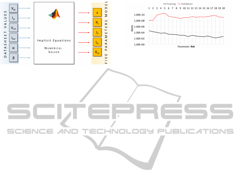
Figure 2: Identiﬁcation of the ﬁve-parameter model by

means of numerical solution of implicit equations system.

nature of the involved equations. Recently, it has been

observed (Laudani et al., 2013) that the ﬁve implicit

equations used in the ﬁve-parameter model identiﬁ-

cation can be manipulated algebraically to reduce the

number of unknowns. In particular, the unknowns of

Irr

, I

and R

can be expressed as a function of the

unknown n = a/N

and R

by means of closed forms

expressions, like:

= h(n,R

) (2)

= f(n,R

) (3)

irr

= g(n,R

) (4)

where the function f(n,R

), g(n,R

) and h(n,R

) are

respectivelygiven by the formulae reported in the Ap-

pendix together with a table summarizing the nomen-

clature. This reduction has two beneﬁts. First, the

problem of model identiﬁcation is reduced to the ex-

traction of only two unknown parameters (n and R

allowing simpler optimization techniques to be used.

Second, differently from the ﬁve-parameter problem,

this is generally a convexunimodal problem. Another

important advantage of the two-parameter model lies

in the search domain. Consider the ﬁve-parameter

model: while a lower bound for the ﬁve parameters

is apparent (i.e. they must be positive to be physically

sensible) the upper bound is undeﬁned. An exception

can be made for the n parameter, deﬁned by solid-

state physics lower than 2 (although often amorphous

silicon modules have higher ideality factor), accord-

ing to the transport mechanism for charges inside the

junction. The remaining four parameters, however,

must be searched in the positive semi-space of solu-

tions. By using the reduced closed forms model, the

unknown is related to I

Irr

, I

and R

by means of

the above cited implicit equations. By imposing the

non-negativity of I

Irr

, I

and R

, it is possible to for-

mulate an upper bound for R

itself. Thus the result-

ing equations with the relative constraints constitutes

an optimization problem easier to address and solve

than the original one inherent in the ﬁve-parameter

Figure 3: Mean error on training and validation for MLP

estimating R

parameter ( hidden layer size up to 20 neu-

rons).

model identiﬁcation (Laudani et al., 2014a; Laudani

et al., 2014b). Nevertheless, the system of the reduced

model still cannot be solved easily outside a suitable

computing environment, such as Matlab, Mathcad,

etc. This drawback has not allowed the development

of suitable management software of PV plants in low

cost computational system (such as microncontroller

based architecture), which is of interest for the pho-

tovoltaic system industry. On the other hand, it al-

lowed the identiﬁcation of thousands of modules from

database in few minutes giving the possibility to con-

stitute a valid dataset for the training of a NN able to

deal with this kind of problem.

3 SET-UP OF THE PV MODEL

NEURAL IDENTIFIER

Different possibilities arises when choosing for a NN

architecture. Firstly, the nature of the problem must

be examined: static or dynamic problems inﬂuence

our choice in the direction of feed forward or recur-

rent networks. In this case, the problem is a static

identiﬁcation problem which can be solved by a feed

forward approach. Another point to take into ac-

count is the complexity of the implementation in low

cost/performance system. Starting from these consid-

erations the Multi-Layer-Perceptron (MLP) architec-

ture is surely the clear choice for this kind of prob-

lems. In the MLP architecture the neurons are orga-

nized in subsequent layers, and the connections are

made using a feed forward conﬁguration: no connec-

tion exists between neurons of the same layer, but

each neuron communicates via weighted connections

to all the neurons of the successive layer. The num-

ber of layers in a MLP is variable, with a minimum of

three. In this case, the Input layer performs no opera-

tions. The Hidden layer is composed by neurons with

a non-linear activation function. The Output layer is

analogous to the second, but with a simple linear acti-

vation function. Indeed, the hidden layer re-maps the

inputs so that they are linearly separable, and the out-

NCTA2014-InternationalConferenceonNeuralComputationTheoryandApplications

132

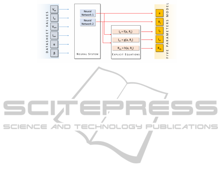
Figure 4: Identiﬁcation of the parameters by means of a neural system and explicit equations.

put layer performs linear combination. By the Univer-

sal Approximation Theorem (Cybenko, 1989; Hornik

et al., 1989) a feed forward neural network with a sin-

gle hidden layer containing a ﬁnite number of neu-

rons can interpolate any continuous function. In ad-

dition, the single hidden layer MLP is a standard ar-

chitecture, where the only parameter is the number of

neurons in the hidden layer. The advantage of this

architecture lies in its univocal determination by the

number of neurons: given the hidden layer size, the

number of inputs and the number of outputs, the NN

architecture is completely deﬁned. Another impor-

tant issue is that the relation between training per-

formance and layer size has been investigated thor-

oughly in literature (Ilonen et al., 2003; Rawat et al.,

2013; Hunter et al., 2012; Teoh et al., 2006; Kim

and Lee, 2008). However, complex problems may

require a very high number of neurons, making the

training of a single hidden layer MLP difﬁcult: that

is, even if the MLP could approximate any function,

it may not be the most efﬁcient way to do it (Wil-

amowski, 2009). On this behalf, different architec-

tures arose in literature. Nevertheless, it usually is

the ﬁrst typology of NN to try when a new problem

is addressed for the ﬁrst time. For the implementa-

tion of the neural identiﬁer of the PV ﬁve parameter

model we have investigated the use of MLP architec-

tures, since we have already successfully used it for

other PV related problems: in particular for the so-

lution of maximum power point identiﬁcation (Car-

rasco et al., 2013) and for the prediction of solar ir-

radiance from PV voltage and current measurements

(Mancilla-David et al., 2014). The approach pursued

in this paper is to use a neural network to estimate

the parameters of the one diode model starting from

datasheet value, as explained in section 2. The sim-

plest strategy would be to substitute the block shown

in ﬁgure 2 with a MLP composed by multiple inputs

and outputs, train it on the training set and validate the

results obtained. It has been observed, however, that

by using a MIMO architecture, an effective estimation

with NN cannot be achieved for the addressed prob-

lem. To understand the reasons behind this behavior,

the MIMO was split in multiple MISO networks (Par-

odi et al., 2012), one for each of the ﬁve parameters

ﬁguring in the model. By trying to compute the pa-

rameters individually, the problem became apparent:

the parameter R

could not be estimated by the NN,

at least by using a low/medium number of neurons,

and consequently neither by the MIMO network (the

performance of the MISO network up to 20 neurons

can be seen in ﬁgure 3). This parameter, by itself,

was the cause of the NN approach failure. This jus-

tiﬁes as well the lack of PV model neural identiﬁers.

By taking advantage of the closed forms proposed in

Section 2, the calculation of parameters I

, R

and

Irr

is not necessary to identify the model. Indeed,

as can be seen in ﬁgure 4, the NN approach can be

used to evaluate the two independent parameters R

and a, while the remaining three can be calculated by

using the closed forms f(n,R

), g(n,R

) and h(n,R

)

(n = a/N

). Thus, two MISO NN have been imple-

mented: both NNs receive as inputs the six datasheet

values (the open circuit voltage of the cell V

, the

short circuit current I

, the voltage and current at the

maximum power point I

MPP

and V

MPP

, and the tem-

perature coefﬁcient of both I

and V

, respectively

and β

.), and returns as output either R

or a.

3.1 Dataset and Training Procedure

Description

The dataset used to train the neural networks in the

present work was acquired from a large database of

panels (California Energy Commission, 2013). The

database collects all the relevant datasheet informa-

tions for about 10000 photovoltaic panels. By using

the techniques illustrated in (Laudani et al., 2014b)

for each module of the database a ﬁve-parameter

model was identiﬁed. In order to verify the gener-

alization capabilities of our neural network, we de-

cided to use the modules with Monocrystalline Sili-

con (mono-Si) technology available on CEC database

ModelIdentificationforPhotovoltaicPanelsUsingNeuralNetworks

133

as training set, and the modules with multicrystalline

Silicon (multi-Si) technology as test set. Choosing

the mono-Si modules should also guarantee a training

dataset capable of representing an acceptable diver-

sity of panels with different characteristics. In addi-

tion, in this way we can assume that the neural iden-

tiﬁer has learnt to solve this system of trascenden-

tal equations, since the two technologies differ sig-

niﬁcantly in the reference parameters. The resulting

training set consists of about 4000 entries, whereas

the test set has more than 6000 modules. The inter-

polation capabilities of a NN can be correlated to the

number of neurons composing the network itself. On

the other hand, an relationship can be achieved for

each kind of problem, which links for a data general-

ization measure the number of neurons with the size

of the training set (more explanations can be found

in (Fulginei et al., 2013) and are out of the scope of

this work). In our case training set is very large with

respect to the number of neurons adopted and conse-

quently it is improbable to run into over trained net-

works. Finally, in our investigation, we adopted the

following principles: i) we use a NN with a number

of neurons in the hidden layer variable from 20 down

to 1; ii) each NN with a ﬁxed number of neurons is

trained 10 times for 1000 epochs in order to perform

a statistical analysis of the results (minimum, average,

median and standard deviation are computed); iii) No

validation set has been used for early stopping tech-

niques. One of the reasons behind the choice of not

using the early stopping mechanism with a validation

set is the low number of epochs adopted with respect

the size of the training set. As stated, each single NN

was trained multiple times, changing the characteris-

tic size and making a statistic analysis of the train-

ing and validation performances for both sets (train-

ing and test data set). A total of 2x10x20 MLP were

trained and validated. The performance was evalu-

ated using as metric the MSE on training (or test) set

and the NNs output. The discussion on the results is

reported in the next section.

4 RESULTS AND DISCUSSION

The performance of the Neural identiﬁer are summa-

rized in the tables 1 and 2 where the minimum MSE

for both training and test set are reported for parame-

ters a and R

, respectively. As it is possible to notice

the MSE reaches extremely low values (under 1E-7)

giving an accurate estimation of these two parame-

ters. It is worth to remind that the training set is made

of mono-Si modules whereas the test set is made of

multi-Si modules: the low MSE achieved on test set

allows us to conﬁrm the generalization capabilities of

the Neural networks. In addition, the MSE decreases

by adding further neurons, and this trend should con-

tinue for a number of neurons higher than 20 in the

Table 1: Result for parameter a.

Neurons min MSE on min MSE

training set on test set

1 5.129E-02 4.133E-02

2 2.827E-04 2.947E-04

3 9.733E-06 5.271E-05

4 2.987E-06 1.461E-05

5 5.597E-07 3.566E-05

6 2.168E-07 3.079E-05

7 1.218E-07 1.312E-05

8 2.657E-08 3.103E-07

9 7.755E-08 5.162E-06

10 2.305E-08 1.233E-05

11 5.416E-09 9.532E-06

12 9.227E-09 9.425E-06

13 1.280E-08 3.649E-06

14 9.672E-09 5.569E-06

15 8.046E-09 1.073E-05

16 1.341E-08 8.131E-06

17 4.077E-09 2.652E-06

18 1.733E-08 6.063E-06

19 1.619E-09 5.078E-07

20 1.218E-09 9.606E-07

Table 2: Result for parameter R

Neurons min MSE on min MSE

training set on test set

1 7.033E-04 4.903E-04

2 6.979E-05 2.619E-05

3 3.844E-06 7.508E-06

4 1.444E-06 1.734E-06

5 3.914E-07 7.847E-07

6 5.802E-08 3.084E-07

7 2.049E-08 1.468E-07

8 5.303E-09 6.925E-08

9 5.316E-09 3.302E-08

10 1.679E-09 2.223E-08

11 1.266E-09 4.499E-08

12 6.415E-10 1.685E-08

13 5.282E-10 1.275E-08

14 3.045E-10 6.508E-09

15 4.748E-10 1.266E-08

16 1.715E-10 9.018E-09

17 1.789E-10 6.829E-09

18 1.919E-10 5.594E-09

19 8.278E-11 2.025E-09

20 1.100E-10 1.096E-08

NCTA2014-InternationalConferenceonNeuralComputationTheoryandApplications

134

hidden layer as well. However accurate results are

already achived with less than 20 neurons and con-

sequently it is not necessary to further add neurons.

In ﬁgures 5 and 6 the comparison between the val-

ues of a and R

parameters and NN output of the best

NNs trained, are shown for the ﬁrst 1000 modules of

the test set. Practically the values returned by NN are

superimposed to the exact values (a maximum differ-

ence of the order of 1E-4 is achieved, which is surely

satisfactory since the input data have a precision lower

than this). This gap is clearly due to the precision of

the trained NN. This could be reduced if we further

train the network by using a high number of epochs.

But, in every case, it is already quite acceptable, con-

sidering that the state of the art approach for this com-

putation used often approximated formulae introduc-

ing error of the order of 1% (see (Cubas et al., 2014;

Li et al., 2013) for reviews of these approaches). At

the same time, from these accurate values, the other

dependent parameters R

, I

and I

Irr

can be com-

puted precisely by using the respective closed forms,

conﬁrming that the use of NN in conjunction with re-

duced closed forms allows to identify quickly the one

diode model. The suggested sizes in both cases is 19

neurons in the hidden layer: this choice is done con-

sidering the MSE complessively obtained for all the

10000 PV modules constituting the training and test

set. Indeed the aim is also to use this NN for the

solution of the problem in a real application and to

implement it in embedded systems, and consequently

we are interested in the best performance available on

all modules with a low computational cost. In this

sense, if we accept a higher error, the NNs with 8 neu-

rons allows to achieve a good accuracy estimation as

well (MSE about 1E-7) with a lower computational

cost. Lastly, it is worth noticing that the comparison

with the other approaches must be done in terms of

both computational cost/environment of implementa-

tion and precision; thus we have: exact methods, such

as those proposed in (Laudani et al., 2014b), which

although efﬁcient cannot be implemented in low cost

microcontroller based system (Mancilla-David et al.,

2014); other high accuracy approaches (such as those

reported in (Li et al., 2013) or based on cluster anal-

ysis (Sandrolini et al., 2010)), which have prohibitive

computational cost; approximated methods, such that

one reported in (Cubas et al., 2014) which introduce

errors in the calculation of the parameters and have

a low computational cost. The approach herein pro-

posed is efﬁcient from the computational cost point

of view and enough correct in the estimation of the

ﬁve-parameter model and thus it is a good trade-off

with respect the approaches presented in literature.

Although the MLP architecture could be not so ef-

100 200 300 400 500 600 700 800 900

module

parameter value

NN output

Figure 5: a parameter values versus estimated by Neural

Networks for 1000 modules of the test set.

ﬁcient, we have veriﬁed that an implementation of

the same problem by using a Full Connected Cascade

NN (Wilamowski, 2009) did not give signiﬁcativeim-

provement in the results and showed an equivalent

computational cost.

5 CONCLUSIONS

A neural network approach to identify PV one diode

model was proposed. The work started from the pre-

liminary analysis of the CEC database, which collects

the datasheet parameters of about 10000 PV panels.

For each panel in the database, the ﬁve parameters

for the classical one-diode model were determined

via numerical approach, creating a training and val-

idation dataset. A ﬁrst approach, consisting of a di-

rect computation of parameters via MIMO NN was

found unsuccessful. Further analysis suggested to

avoid predicting all the parameters, and instead, use

the NN approach just on the independent ones. Then,

two MLP were used to interpolate the two param-

eters. From the obtained results, it is obvious that

100 200 300 400 500 600 700 800 900

0.2

0.4

0.6

0.8

1.2

module

parameter value

NN output

Figure 6: R

parameter values versus estimated on by Neu-

ral Networks for 1000 modules of the test set.

ModelIdentificationforPhotovoltaicPanelsUsingNeuralNetworks

135

in literature the neural network approach was often

overlooked because of the hard obstacle encountered

in the prediction of the shunt resistance. The solu-

tion of switching to closed forms for the identiﬁcation

of the model, shifts the problem of the shunt resis-

tance calculus to the solution of an explicit non-linear

equation. In conclusion, NNs can identify the R

and

a parameters correctly, making the NN approach vi-

able for model identiﬁcation in conjunction with the

adoption of reduced forms for the computation of the

three remaining unknown parameters of the one diode

model. The so achieved NN for the estimation of the

series resistance R

and the modiﬁed ideality factor

a, and the closed form for the computation of the re-

maining dependent parameters constitute a complete

tool extremely easy to be implemented in a microcon-

troller based architecture: this is another successful

step made thanks to Soft Computing techniques in the

development of intelligent systems for the monitoring

and the management of renewable generation plants.

REFERENCES

Askarzadeh, A. and Rezazadeh, A. (2013). Artiﬁcial bee

swarm optimization algorithm for parameters iden-

tiﬁcation of solar cell models. Applied Energy,

102(0):943 – 949.

Blair, N. J., Dobos, A. P., and Gilman, P. (2010). Com-

parison of photovoltaic models in the system advisor

model. In Solar 2013, Baltimore, Maryland.

California Energy Commission (2013). CECPV

calculator version 4.0. [Online]. Avialable:

http://www.gosolarcalifornia.org/tools/nshpcalculator/.

Capizzi, G., Coco, S., Giuffrida, C., and Laudani, A. (2004).

A neural network approach for the differentiation of

numerical solutions of 3-d electromagnetic problems.

Magnetics, IEEE Transactions on, 40(2):953–956.

Carrasco, M., Mancilla-David, F., Fulginei, F. R., Laudani,

A., and Salvini, A. (2013). A neural networks-based

maximum power point tracker with improved dynam-

ics for variable dc-link grid-connected photovoltaic

power plants. International Journal of Applied Elec-

tromagnetics and Mechanics, 43(1).

Cubas, J., Pindado, S., and Victoria, M. (2014). On the an-

alytical approach for modeling photovoltaic systems

behavior. Journal of Power Sources, 247:467 – 474.

Cybenko, G. (1989). Approximation by superpositions of

a sigmoidal function. Mathematics of control, signals

and systems, 2(4):303–314.

Desoto, W., Klein, S., and Beckman, W. (2006). Improve-

ment and validation of a model for photovoltaic array

performance. Solar Energy, 80(1):78–88.

El-Naggar, K., AlRashidi, M., AlHajri, M., and Al-Othman,

A. (2012). Simulated annealing algorithm for pho-

tovoltaic parameters identiﬁcation. Solar Energy,

86(1):266 – 274.

Fulginei, F. R., Laudani, A., Salvini, A., and Parodi, M.

(2013). Automatic and parallel optimized learning

for neural networks performing MIMO applications.

Advances in Electrical and Computer Engineering,

13(1):3–12.

Hornik, K., Stinchcombe, M., and White, H. (1989). Multi-

layer feedforward networks are universal approxima-

tors. Neural networks, 2(5):359–366.

Hunter, D., Yu, H., Pukish, M. S., Kolbusz, J., and Wil-

amowski, B. M. (2012). Selection of proper neural

network sizes and architectures - A comparative study.

Industrial Informatics, IEEE Trans. on, 8(2):228–240.

Ilonen, J., Kamarainen, J.-K., and Lampinen, J. (2003).

Differential evolution training algorithm for feed-

forward neural networks. Neural Processing Letters,

17(1):93–105.

Ishaque, K. and Salam, Z. (2011). An improved modeling

method to determine the model parameters of photo-

voltaic (PV) modules using differential evolution (de).

Solar Energy, 85(9):2349 – 2359.

Jiang, L. L., Maskell, D. L., and Patra, J. C. (2013). Pa-

rameter estimation of solar cells and modules using

an improved adaptive differential evolution algorithm.

Applied Energy, 112(0):185 – 193.

Kim, C.-T. and Lee, J.-J. (2008). Training two-layered feed-

forward networks with variable projection method.

Neural Networks, IEEE Trans. on, 19(2):371–375.

Laudani, A., Fulginei, F. R., and Salvini, A. (2014a). High

performing extraction procedure for the one-diode

model of a photovoltaic panel from experimental I–V

curves by using reduced forms. Solar Energy, 103:316

– 326.

Laudani, A., Fulginei, F. R., Salvini, A., Lozito, G. M., and

Coco, S. (2014b). Very fast and accurate procedure

for the characterization of photovoltaic panels from

datasheet information. International Journal of Pho-

toenergy, 2014. Article ID 946360.

Laudani, A., Mancilla-David, F., Riganti-Fulginei, F., and

Salvini, A. (2013). Reduced-form of the photovoltaic

ﬁve-parameter model for efﬁcient computation of pa-

rameters. Solar Energy, 97(0):122 – 127.

Li, Y., Huang, W., Huang, H., Hewitt, C., Chen, Y., Fang,

G., and Carroll, D. L. (2013). Evaluation of methods

to extract parameters from currentvoltage characteris-

tics of solar cells. Solar Energy, 90(0):51 – 57.

Liu, Y.-H., Liu, C.-L., Huang, J.-W., and Chen, J.-H.

(2013). Neural-network-based maximum power point

tracking methods for photovoltaic systems operating

under fast changing environments. Solar Energy,

89:42–53.

Mancilla-David, F., Riganti-Fulginei, F., Laudani, A., and

Salvini, A. (2014). A neural network-based low-cost

solar irradiance sensor. Instrumentation and Measure-

ment, IEEE Trans. on.

Parodi, M., Fulginei, F. R., and Salvini, A. (2012). Learn-

ing optimization of neural networks used for mimo ap-

plications based on multivariate functions decomposi-

tion. Inverse Problems in Science and Engineering,

20(1):29–39.

Rajasekar, N., Kumar, N. K., and Venugopalan, R. (2013).

NCTA2014-InternationalConferenceonNeuralComputationTheoryandApplications

136

Bacterial foraging algorithm based solar {PV} param-

eter estimation. Solar Energy, 97(0):255 – 265.

Rawat, R., Patel, J. K., and Manry, M. T. (2013). Mini-

mizing validation error with respect to network size

and number of training epochs. In Neural Networks

(IJCNN), The 2013 International Joint Conference on,

pages 1–7. IEEE.

Sandrolini, L., Artioli, M., and Reggiani, U. (2010). Nu-

merical method for the extraction of photovoltaic

module double-diode model parameters through clus-

ter analysis. Applied Energy, 87(2):442 – 451.

Siddiqui, M. and Abido, M. (2013). Parameter estimation

for ﬁve- and seven-parameter photovoltaic electrical

models using evolutionary algorithms. Applied Soft

Computing, 13(12):4608 – 4621.

Teoh, E., Tan, K., and Xiang, C. (2006). Estimating the

number of hidden neurons in a feedforward network

using the singular value decomposition. Neural Net-

works, IEEE Trans. on, 17(6):1623–1629.

Wilamowski, B. M. (2009). Neural network architectures

and learning algorithms. Industrial Electronics Mag-

azine, IEEE, 3(4):56–63.

Xu, C., Wang, C., Ji, F., and Yuan, X. (2012). Finite-

element neural network-based solving 3-d differential

equations in mﬂ. Magnetics, IEEE Transactions on,

48(12):4747–4756.

Yadav, A. K. and Chandel, S. (2014). Solar radiation pre-

diction using artiﬁcial neural network techniques: A

review. Renewable and Sustainable Energy Reviews,

33:772 – 781.

Zagrouba, M., Sellami, A., Bouacha, M., and Ksouri, M.

(2010). Identiﬁcation of PV solar cells and mod-

ules parameters using the genetic algorithms: Appli-

cation to maximum power extraction. Solar Energy,

84(5):860 – 866.

APPENDIX

In this appendix we summarize the main symbols

and formulae useful for understanding the one-diode

model and its reduced form. In particular table 3 re-

ports the nomenclature used and the deﬁnition of pa-

rameters. With the aim to simplify the notation and

the expressions, the shunt conductance G

= R

−1

will be used instead of R

, and the following quanti-

(

− )[ ( + − − ) + ]

[( + − ) − ]

(8)

( − 2 )

( − )[ ( + − − ) + ]

(9)

[ ( − + ) + (2 (1 − ) − )]

( − )[ ( + − − ) + ]

(10)

Table 3: List of the technical parameters used in this work.

Name Value or Description

S Irradiance

T Cell temperature

n Ideality factor

a N

Number of series modules/cells

ref

◦

C at SRC

ref

1000

at SRC

Series resistance at SRC

Irr

Photocurrent at SRC

Reverse saturation current at SRC

Shunt resistance at SRC

−1

Open circuit voltage at SRC

Short circuit current at SRC

MPP

Maximum power voltage at SRC

MPP

Maximum power current at SRC

Temperature coeff. for I

Temperature coeff. for V

ties are deﬁned:

EXP

= exp





(5)

EXP

MPP

= exp



MPP

+ R

MPP



(6)

EXP

= exp





(7)

The formulae (2),(3) and (4), which express R

, I

and I

irr

as function of R

and modiﬁed ideality factor

a are respectively (8), (9) and (10).

ModelIdentificationforPhotovoltaicPanelsUsingNeuralNetworks

137

REFERENCES

Askarzadeh, A. and Rezazadeh, A. (2013). Artificial bee