
Sliding Mode Control of Linear Time-varying Systems
Application to Trajectory Tracking Control of Nonlinear Systems
Yasuhiko Mutoh and Nao Kogure
Department of Engineering and Applied Sciences, Sophia University, 7-1 Kioicho, Chiyoda-ku, Tokyo, Japan
Keywords:
Sliding Mode Control, Linear Time-varying System, Non-linear System, Tracking Control.
Abstract:
This paper concerns with the sliding mode controller design method for linear time-varying systems. For
this purpose, using the time-varying pole placement technique, the state feedback is designed first so that the
time-varying closed loop system is equivalent to the standard linear time invariant system. Then, conventional
sliding mode controller design method is applied to this time invariant system to obtain the control input.
Finally, using the time-varying transformation matrix, this sliding mode control input is put back to the control
input for the original system. In this paper, this controller is applied to the trajectory tracking control problem
for nonlinear systems.
1 INTRODUCTION
This paper concerns with the sliding mode controller
design for linear time varying systems, and then, we
apply this control technique to a trajectory tracking
control of non-linear systems.
The author proposed the simple design method of
the pole placement controller for linear time varying
systems using the concept of the relative degree of
the system (Mutoh,2011) (Mutoh and Kimura,2011).
This pole placement design purpose is to make the
time varying closed loop system equivalent to some
linear time invariant system that has desired eigenval-
ues, by the state feedback. In this paper, we make use
of this technique for designing the sliding mode con-
troller for linear time varying systems. The first step
is to find the state feedback for the linear time varying
system so that the closed loop system is equivalent to
some linear time-invariant standard system. Then, by
using the conventional sliding mode controller design
method, the sliding mode control input for this linear
time invariant system can be obtained (Utkin,1992).
After that, using an equivalent time varying transfor-
mation matrix, this control input can be transformed
into the sliding mode control for the original linear
time varying system. Since, the sliding mode con-
troller is designed for the equivalent time invariant
system, any type of conventional sliding mode con-
troller design method can be applied.
If we need to control nonlinear systems to follow
some particular desired trajectory in wide range, the
most simple idea might be to approximate the nonlin-
ear system along this trajectory using a linear time-
varying system. However, since, controller design
method for linear time-varying system is not neces-
sarily simple, it seems that this approach is not com-
monly used. In this paper, the abovetime varyingslid-
ing mode control technique is applied to the trajectory
tracking control problem of non-linear systems. Some
simulation results will be also shown.
2 PRELIMINARIES
In this section, the basic properties of linear time-
varying systems which we will use later are presented.
Consider the following linear time-varying multi-
input system.
˙x(t) = A(t)x(t) + B(t)u(t) (1)
Here, x(t) ∈ R
n
and u(t) ∈ R
m
are the state variable
and the input signal, respectively. A(t) ∈ R
n×n
and
B(t) ∈ R
n×m
are time varying coefficient matrices,
which are bounded and smooth functions of t.
The matrix B(t) is written as follows, using col-
umn vectors b
i
(t) ∈ R
n
(i = 1, ·· · , m).
B(t) =
b
1
(t) b
2
(t) ··· b
m
(t)
(2)
Let b
i
k
(t) ∈ R
n
be defined by the following recur-
492
Mutoh Y. and Kogure N..
Sliding Mode Control of Linear Time-varying Systems - Application to Trajectory Tracking Control of Nonlinear Systems.
DOI: 10.5220/0005019704920498
In Proceedings of the 11th International Conference on Informatics in Control, Automation and Robotics (ICINCO-2014), pages 492-498
ISBN: 978-989-758-039-0
Copyright
c
2014 SCITEPRESS (Science and Technology Publications, Lda.)

sive equations.
b
0
k
(t) = b
k
(t)
b
i
k
(t) = A(t)b
i−1
k
(t) −
˙
b
i−1
k
(t)
(3)
k = 1, 2· ·· m, i = 1, 2···
Then, the controllability matrix of the system (1) can
be written as follows.
U
c
= [b
0
1
(t)· ·· b
0
m
(t)|· ·· |b
n−1
1
(t)· ·· b
n−1
m
(t)] (4)
Theorem 1. The system (1) is completely control-
lable if and only if
rankU
c
(t) = n
∀
t (5)
If the system (1) is completely controllable, we
can define the controllability indices, µ
1
, µ
2
,·· ·, µ
m
,
which satisfy the following equations,
R(t) : nonsingular
m
∑
i=1
µ
i
= n (6)
where
R(t) =
h
b
0
1
(t)· ·· b
µ
1
−1
1
(t)|· ·· |b
0
m
(t)· ·· b
µ
m
−1
m
(t)
i
(7)
which is called the truncated controllability matrix.
In this paper, it is assumed that if the system is com-
pletely controllable, its controllability indices satisfy
the inequality, µ
1
≥ µ
2
≥ ··· ≥ µ
m
, without loss of
generality.
Definition 1. Consider the following output equation
for the system (1),
y(t) = C(t)x(t) (8)
Here, y(t) ∈ R
m
is some output signal and C(t) ∈
R
m×n
is a time varying coefficient matrices. Let p be
a differential operator. System (1)(8) has the vector
relative degree, r
1
, r
2
, · ·· , r
m
from u to y, if there ex-
ist some matrix D(t) ∈ R
m×n
and some nonsingular
matrix Λ(t) ∈ R
m×m
, such that
p
r
1
.
.
.
p
r
m
y(t) = D(t)x(t) + Λ(t)u(t). (9)
It should be noted that p
r
i
can be replaced by arbitrary
monic polynomial of p of degree r
i
. ∇
3 STANDARD TIME INVARIANT
SYSTEM
To design the sliding mode controller for the system
(1), we first design the state feedback with a new input
vector v(t) ∈ R
m
, so that the closed loop system is
equivalent to the linear time invariant standard form.
Suppose that the system (1) is completely control-
lable. Then, if
˜
C(t) ∈ R
m×n
is defined by
˜
C(t) = W(t)R
−1
(t) (10)
where
W(t) = diag(w
1
(t), w
2
(t), · ·· , w
m
(t))
w
i
(t) = [0, · ·· , 0, λ
i
(t)] ∈ R
1×µ
i
(i = 1, · ·· , m)
λ
i
(t) 6= 0
(11)
and also if a new output signal ˜y(t) ∈ R
m
is defined by
˜y(t) =
˜
C(t)x(t) (12)
then, the vector relative degree from u(t) to ˜y(t) is
µ
1
, µ
2
, ··· , µ
m
(Mutoh and Kimura,2011).
Let ˜y(t) and
˜
C(t) be
˜y(t) =
˜y
1
(t)
.
.
.
˜y
m
(t)
,
˜
C(t) =
˜c
1
(t)
.
.
.
˜c
m
(t)
. (13)
By differentiating ˜y(t) successively, we have
˜y
i
(t) = ˜c
0
i
(t)x(t)
˙
˜y
i
(t) = ˜c
1
i
(t)x(t)
¨
˜y
i
(t) = ˜c
2
i
(t)x(t)
.
.
.
˜y
(µ
i
)
i
(t) = ˜c
µ
i
i
(t)x(t) + ˜c
µ
i
−1
i
(t)B(t)u(t)
= ˜c
µ
i
i
(t)x(t) + λ
i
(t)u
i
(t)
+ γ
i(i+1)
u
i+1
··· + γ
im
(t)u
m
(t)
i = 1, · ·· , m (14)
Here, ˜c
j
i
(t) and γ
ij
(t) are obtained by the following
recursive equation from
˜
C(t).
˜c
0
i
(t) = ˜c
i
(t)
˜c
j+1
i
(t) = ˜c
j
i
(t)A(t) +
˙
˜c
j
i
(t)
(15)
i = 1, 2· ·· m, j = 1, 2· ··
and
γ
ij
(t) = c
µ
i
−1
i
(t)b
j
(t). (16)
Hence, from (14), we have
p
µ
1
.
.
.
p
µ
m
˜y(t) = D(t)x(t) + Λ(t)u(t)
(17)
where,
D(t) =
˜c
µ
1
1
(t)
˜c
µ
2
2
(t)
.
.
.
˜c
µ
m
m
(t)
, Λ(t) =
Λ
1
(t)
Λ
2
(t)
.
.
.
Λ
m
(t)
(18)
SlidingModeControlofLinearTime-varyingSystems-ApplicationtoTrajectoryTrackingControlofNonlinearSystems
493
and
Λ
i
(t) = [0, ·· · , 0, λ
i
(t), γ
i(i+1)
(t), · ·· , γ
ij
(t)] (19)
Thus, by the state feedback
u(t) = Λ
−1
(t)(−D(t)x(t) + v(t)) (20)
with the new input signal v(t) ∈ R
m
, the closed loop
system becomes
p
µ
1
.
.
.
p
µ
m
˜y(t) = v(t). (21)
This system has the following state realization.
˙
ω(t) = A
∗
ω(t) + B
∗
v(t)
=
A
∗
1
0
.
.
.
0 A
∗
m
ω(t)
+
b
∗
1
··· 0
.
.
.
0 ··· b
∗
m
v(t) (22)
where ω(t) ∈ R
n
, A
∗
∈ R
n×n
, B
∗
∈ R
n×m
, and
A
∗
i
=
0 1 0
.
.
.
.
.
.
.
.
.
.
.
. 1
0 0 . . . 0
∈ R
µ
i
×µ
i
(i = 1, . . . , m) (23)
b
∗
i
=
0
.
.
.
0
1
∈ R
µ
i
.
The system (22)(23) is called the linear time invariant
standard form. This new state variable ω(t) ∈ R
n
is
defined by
ω(t) =
˜y
1
(t)
.
.
.
˜y
(µ
1
−1)
1
(t)
.
.
.
˜y
m
(t)
.
.
.
˜y
(µ
m
−1)
m
(t)
. (24)
From (14), the original state variable x(t) and ω(t)
satisfy the relation
ω(t) = T(t)x(t) (25)
where the transformation matrix, T(t), is defined by
T(t) =
˜c
0
1
(t)
.
.
.
˜c
µ
1
−1
1
(t)
.
.
.
˜c
0
m
(t)
.
.
.
˜c
µ
m
−1
m
(t)
. (26)
4 SLIDING MODE CONTROLLER
DESIGN
4.1 Controller for Linear Time-varying
Systems
In this section, the sliding mode controller design
for the linear time varying system (1) is presented.
For this purpose, we first design the sliding mode
control input v(t) for the linear time invariant sys-
tem (22)(23), and then, transform v(t) into the sliding
mode control input for the original system (1), using
the relation (25)(26).
If we write ω(t) and v(t) as
ω(t) =
ω
1
(t)
.
.
.
ω
m
(t)
, ω
i
(t) ∈ R
µ
i
v(t) =
v
1
(t)
.
.
.
v
m
(t)
(27)
(i = 1, ··· , m)
the system (22)(23) is presented as following m sub-
systems.
˙
ω
i
(t) =
0 1 ··· 0
.
.
. ·· ·
.
.
.
.
.
.
0 ··· 0 1
0 ··· · ·· 0
ω
i
(t) +
0
.
.
.
0
1
v
i
(t)
(i = 1, ··· , m) (28)
Since the system (28) is the standard form, the design
procedure of the ordinary sliding mode controller is
very simple stated as follows. First, divide ω
i
(t) into
two part.
ω
i
(t) =
ω
i
(t)
ω
µ
i
i
(t)
(29)
ICINCO2014-11thInternationalConferenceonInformaticsinControl,AutomationandRobotics
494

where ω
i
(t) ∈ R
µ
i
−1
and ω
µ
i
i
(t) ∈ R. Then, the sliding
surface is defined by
S
i
ω
i
(t) =
s
i
ω
i
(t) + ω
µ
i
i
(t) = 0 (30)
where
S
i
= [s
i
, 1] ∈ R
1×µ
i
, s
i
∈ R
1×(µ
i
−1)
(i = 1, · ·· , m). (31)
From (28),(29) and (30), the dynamics on the i-th slid-
ing surface becomes
˙
ω
i
(t) =
0 1 0 ··· 0
0 0 1 ··· 0
.
.
. ·· · ·· ·
.
.
.
.
.
.
0 ··· ··· 0 1
−s
i
ω
i
(t). (32)
From the above, if the desired stable characteristic
polynomial of the i-th sliding dynamics is chosen as
α
i
(p) = p
µ
i
−1
+ α
i
µ
i
−2
p
µ
i
−2
+ · ·· + α
i
0
(33)
then, the i-th sliding surface is
S
i
ω
i
(t) = [ α
i
0
, ··· , α
i
µ
i
−2
, 1 ]ω
i
(t) = 0. (34)
Since, the i-th subsystem is
˙
ω
i
(t) = A
∗
i
ω
i
(t) + b
∗
i
v
i
(t) (35)
it is well known that the i-th sliding control input v
i
(t)
can be defined by
v
i
(t) = −(S
i
b
∗
i
)
−1
{S
i
A
∗
i
ω
i
(t) + q
i
sgn(σ
i
) + k
i
f
i
(σ
i
)}
(36)
where
σ
i
= S
i
ω
i
(t) (37)
and q
i
> 0 and k
i
> 0 are constant parameters and
f
i
(σ
i
) is a function such that σ
i
f
i
(σ
i
) > 0. In fact, it is
readily shown that, using (36), we have the following
Lyapunov function.
V =
1
2
m
∑
i=1
σ
2
i
> 0,
˙
V =
m
∑
i=1
σ
i
˙
σ
i
< 0 (38)
Using (23), v
i
(t) in (36) becomes
v
i
(t) = −{[0, α
i
0
, ··· , α
i
µ
i
−2
]ω
i
(t)
+q
i
sgn(σ
i
) + k
i
f
i
(σ
i
)}. (39)
Hence, from (25)(26), the sliding mode control input
u(t) for the original system becomes as follows.
u(t) = Λ
−1
(t)(−D(t)x(t) + v(t)) (40)
here
v(t) =
v
1
(t)
.
.
.
v
m
(t)
v
i
(t) = −{[0
s]T
i
(t)x(t) + q
i
sgn(σ
i
) + k
i
f
i
(σ
i
)}
σ
i
= S
i
T
i
(t)x(t)
(i = 1, ··· , m) (41)
where
T
i
(t) =
˜c
0
i
(t)
.
.
.
˜c
µ
i
−1
i
(t)
. (42)
From the above, the design procedure of the slid-
ing mode controller for the system (1) is summarized
as the following steps.
[Design procedure]
STEP 1. Using the controllability matrix, U
c
(t) in
(4), check the controllability of the system (1). If
the system is controllable, calculate the controlla-
bility indices µ
1
, ··· , µ
m
and the truncated control-
lability matrix R(t) in (7).
STEP 2. From (10)(11), calculate
˜
C(t).
STEP 3. Using the recursive equation (15), ob-
tain ˜c
j
i
(t) and, using (16), calculate γ
ij
(t) (i =
1, · ·· , m j = i+ 1, · ·· , m). Then, using (18)(19),
define D(t) and Λ(t).
STEP 4. Using (26) (or (42)), calculate T(t) (or
T
i
(t)).
STEP 5. Define the desired stable characteristic
polynomial (33). Then, define
S
i
= [
s
i
, 1]
s
i
= [ α
i
0
, ··· , α
i
µ
i
−2
] (43)
(i = 1, · ·· , m)
STEP 6. The sliding mode control input is obtained
by (40)(41) and (42).
4.2 Trajectory Tracking Controller for
Nonlinear Systems
In this paper, sliding mode controller for linear time-
varying systems is concerned so far. However, in
practice, we can hardly find any system that can be
modeled by a linear time-varying system. And, the
most of practical systems are nonlinear systems. So,
one of the most important application of the control
problem for linear time-varying systems is a control
design problem of linear time varying approximate
model around some particular trajectory of nonlinear
systems.
Consider the following non-linear system.
˙x(t) = f(x(t), u(t)) (44)
Here, x(t) ∈ R
n
and u(t) ∈ R
m
are the state variable
and the input signal. Let x
∗
(t) and u
∗
(t) be some
particular desired trajectory and the desired input for
x
∗
(t).
SlidingModeControlofLinearTime-varyingSystems-ApplicationtoTrajectoryTrackingControlofNonlinearSystems
495

The problem is to design a controller to track this
desired trajectory x
∗
(t) stably around it. This can be
done by stabilizing this trajectory in the neighborhood
of x
∗
(t) and u
∗
(t). Let ∆x(t) and ∆u(t) be defined by
∆x(t) = x(t) − x
∗
(t)
∆u(t) = u(t) − u
∗
(t).
Then, we have a linear time-varying approximation
around x
∗
(t) and u
∗
(t) as follows.
∆˙x(t) = A(t)∆x(t) + B(t)∆u(t) (45)
A(t) =
∂
∂x
f(x
∗
(t), u
∗
(t))
B(t) =
∂
∂u
f(x
∗
(t), u
∗
(t))
(46)
Then, using time-varying sliding mode control tech-
nique, error equation can be stabilized around the de-
sired trajectory x
∗
(t) and u
∗
(t).
5 NUMERICAL EXAMPLE
Consider the following nonlinear system with two in-
put.
x
1
(t) = x
2
(t)
x
2
(t) = 0.5(1− x
2
1
(t))x
2
(t) − x
1
(t)x
3
(t) + u
1
(t)
x
3
(t) = x
2
1
(t) − x
3
(t) + u
1
(t) + u
2
(t) (47)
Let the desired trajectory x
∗
(t) for this system be
˙x
∗
1
(t) = cost
˙x
∗
2
(t) = −sint
˙x
∗
3
(t) = 1. (48)
Then, the desired input u
∗
(t) for x
∗
(t) is obtained as
follows.
u
∗
1
(t) = 0.5sint(1− cos
2
t)
u
∗
2
(t) = −cos
2
t + 1− u
∗
1
(t) (49)
A linear time-varying approximation of the system
(47) around x
∗
(t) and u
∗
(t) becomes as follows.
d
dt
∆x
1
(t)
∆x
2
(t)
∆x
3
(t)
= A(t)
∆x
1
(t)
∆x
2
(t)
∆x
3
(t)
+B(t)
∆u
1
(t)
∆u
2
(t)
(50)
where
A(t) =
0 1 0
cost sint − 1 0.5sin
2
t −cost
2cost 0 −1
(51)
B(t) =
0 0
1 0
1 1
. (52)
The sliding mode control input to stabilize the sys-
tem (50) can be obtained according to the following
steps.
STEP 1. The controllability matrix,U
c
(t), of the sys-
tem (50)-(52) is
U
c
(t) =
0 0
1
1 0
0.5sin
2
t − cost
1 1
−1
0
···
−cost
···
−1 ···
. (53)
This implies that the system (50)-(52) is control-
lable, and the controllability indices are µ
1
= 2
and µ
2
= 1.
STEP 2. From STEP 1, the truncated controllability
matrix, R(t), becomes
R(t) =
0 1 0
1
1
2
(sin
2
t − 2cost) 0
1 −1 1
.(54)
And from (10)(11), we have
˜
C(t) = W(t)R
−1
(t)
=
0 1 0
0 0 1
−0.5sin
2
t + cost 1 0
1 0 0
1+ 0.5sin
2
t − cost −1 1
=
1 0 0
1+ 0.5sin
2
t − cost −1 1
(55)
where we choose λ
1
(t) = λ
2
(t) = 1.
STEP 3. From (15) and (16), we have following
˜c
k
i
(t) and γ
ij
(t).
˜c
1
1
(t) =
0 1 0
˜c
2
1
(t) =
cost sint − 1
0.5sin
2
t −cost
˜c
1
2
(t) =
sint + 2cost + 1
1− cost cost − 1
γ
12
(t) = 0
And, from these equations, D(t) and Λ(t) are cal-
culated as follows.
D(t) =
cost sint − 1
sint + 2cost + 1
0.5sin
2
t −cost
1− cost cost − 1
(56)
Λ(t) =
λ
1
γ
12
0 λ
2
=
1 0
0 1
ICINCO2014-11thInternationalConferenceonInformaticsinControl,AutomationandRobotics
496
STEP 4. Using (26), the state transformation matrix,
T(t), is
T(t) =
T
1
(t)
T
2
(t)
. (57)
where
T
1
(t) =
1 0 0
0 1 0
. (58)
T
2
(t) =
1+ 0.5sin
2
t − cost −1 1
.
(59)
STEP 5. From (33) and the fact that µ
1
= 2, µ
2
= 1,
we choose
α
1
(p) = p+ 1. (60)
In this case, there is not α
2
(p), because ω
2
(t) is a
scalar. From this, we define
S
1
= [ 1 1 ], S
2
= [ 1 ]. (61)
STEP 6. From the above and (40)(41), the sliding
mode control input is obtained as follows.
u
1
(t) = (1− sint cost)∆x
1
(t) − 0.5sin
2
t∆x
2
(t)
+cost∆x
3
(t) − sgn(σ
1
) (62)
u
2
(t) = −(sint + 2cost + 1)∆x
1
(t)
+(cost − 1)∆x
2
(t) + (1− cost)∆x
3
(t)
−sgn(σ
2
) (63)
where σ
1
and σ
2
are defined by
σ
1
= ∆x
1
(t) + ∆x
2
(t)
σ
2
= (1+ 0.5sin
2
t − cost)∆x
1
(t)
−∆x
2
(t) + ∆x
3
(t). (64)
and q
1
= q
2
= 1, k
1
= k
2
= 0.
Figure 1: Response of ∆x(t).
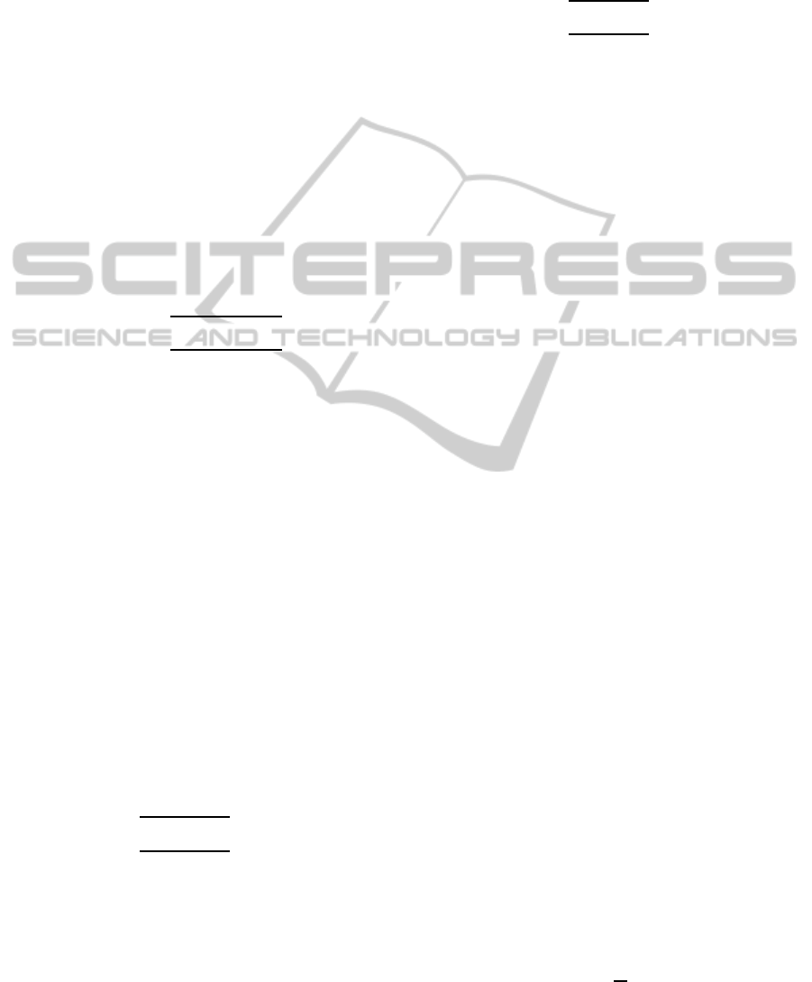
Figure 2: Response of σ = σ
2
1
+ σ
2
2
.
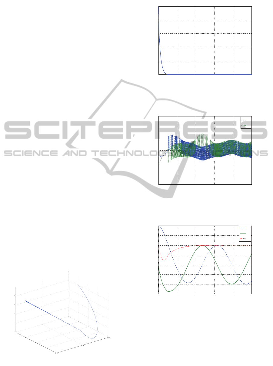
Figure 3: Response of ∆u(t).
Figure 4: Response of x(t).
Fig.1 shows that the response of ∆x(t) which con-
verges to the origin. This implies that the state x(t)
converges to the desired trajectory x
∗
(t).The value of
σ
2
1
+ σ
2
2
is plotted in Fig.2. It decreases monotoni-
cally to 0. Fig.3 and 4 show the control input u(t) and
state response x(t). According to these graphs, the
time varying sliding mode controller works well for
the trajectory tracking control for non-linear systems.
SlidingModeControlofLinearTime-varyingSystems-ApplicationtoTrajectoryTrackingControlofNonlinearSystems
497

6 CONCLUSIONS
In this paper, the design procedure of sliding mode
controller for linear time-varying system is presented.
For this purpose, the time-varying pole placement
feedback is used so that the closed loop system is
equivalent to some linear time invariant system. Then,
the conventional design method of the sliding mode
control can be applied to this time invariant system.
And, finally by the time-varying transformation ma-
trix, this control input is transformed into the sliding
mode control input for the original system. It was
shown that this controller has a good availability for
the trajectory tracking control problem of nonlinear
systems.
REFERENCES
Chi-Tsong Chen (1999)C Linear System Theory and Design
(Third edition). OXFORD UNIVERSITY PRESS
Charles C. Nguyen (1987)C Arbitrary eigenvalue assign-
ments for linear time-varying multivariable control
systems. International Journal of Control, 45-3, 1051–
1057
W.J.Rugh (1993) Linear System Theory 2nd Edition pren-
tice hall
Y.Mutoh (2011)C A New Design Procedure of the Pole-
Placement and the State Observer for Linear Time-
Varying Discrete Systems. Informatics in Control, Au-
tomation and Robotics, p.321-334, Springer
Michael Val´aˇsek (1995)C Efficient Eigenvalue Assignment
for General Linear MIMO systems. Automatica, 31-
11, 1605–1617
Michael Val´aˇsek, Nejat Olgac¸ (1999)C Pole placement
for linear time-varying non-lexicographically fixed
MIMO systems. Automatica, 35-1, 101–108
Y.Mutoh and Kimura (2011)C Observer-Based Pole Place-
ment for Non-Lexicographically-fixed Linear Time-
Varying Systems. 50th IEEE CDC and ECC
V.Utkin (1992), Sliding Mode in Control and Optimization,
Springer-Verlag
A.Poznyak and Y.Shtessel(2003), Min-Max Sliding-Mode
Control for Multimodel Linear Time Varying Sys-
tems, IEEE trans. on Automatic Control, vol.48,
no.12, pp.2141-2150
M.Otsuki,Y.Ushijima,K.Yoshida,H.Kimura,
T.Nakagawa(2005), Nonstationary Sliding Mode
Control Using Time-varying Switching Hyperplane
for Transverse Vibration of Elevator Rope, Proc. of
2005 ASME, Longbeach, USA
ICINCO2014-11thInternationalConferenceonInformaticsinControl,AutomationandRobotics
498
