Receiver Design for an Optical MIMO Testbed

Heidi K¨ohnke, Robert Schwinkendorf, Sebastian Daase, Andreas Ahrens and Steffen Lochmann

Hochschule Wismar, University of Technology, Business and Design, Philipp-M¨uller-Straße 14, 23966 Wismar, Germany

Keywords:

Multiple-input Multiple-output System, Optical Fibre Transmission, Multimode Fiber (MMF), Mode Cou-

pling.

Abstract:

Within the last years multiple-input multiple-output (MIMO) systems have attracted a lot of attention in the

optical ﬁbre community. Although the theoretical background of MIMO transmission is well understood, there

is still a need for practical investigations regarding mode combining, mode maintenance and mode splitting.

Since these components represent an essential part of an optical MIMO system, in this work a (2× 2) MIMO

testbed using fusion couplers and a multi-mode ﬁbre (MMF) length of 1.9 km is set up for an operating

wavelength of 1326 nm. Together with the MIMO receiver-side signal processing the successful transmission

of parallel data streams is presented.

1 INTRODUCTION

The growing demand of bandwidth particularly

driven by the developing Internet has been satisﬁed

so far by optical ﬁbre technologies such as Dense

Wavelength Division Multiplexing (DWDM), Polar-

ization Multiplexing (PM) and multi-level modula-

tion. These technologies have now reached a state

of maturity (Winzer, 2012). The only way to fur-

ther increase the available data rate is now seen in the

area of spatial multiplexing (Richardson et al., 2013),

which is well-established in wireless communications

(Tse and Viswanath, 2005; K¨uhn, 2006). Nowadays

several novel techniques such as Mode Group Diver-

sity Multiplexing (MGDM) (Franz and Blow, 2012)

or Multiple-Input Multiple-Output (MIMO) are in the

focus of interest (Singer et al., 2008).

Among these techniques, optical MIMO has

shown its capability for high-speed data transmission.

However, the practical implementation has to cope

with many technological obstacles such as mode mul-

tiplexing and management. This includes mode com-

bining, mode maintenance and mode splitting.

In order to investigate these effects in a whole

transmission system a MIMO testbed has been set

up. Here, fusion couplers are used for mode combin-

ing and splitting realizing a parallel data transmission

over a 1.9 km multi-mode ﬁbre (MMF) (Ahrens and

Lochmann, 2013; Sandmann et al., 2014a; Sandmann

et al., 2014b). For the necessary implementation of

the MIMO signal processing an off-line MIMO re-

ceiver has been programmed.

Against this background the novelty of this paper

is the practical receiver implementation within a (2×

2) MIMO testbed using fusion couplers. Its proper

mode of operation is shown by the eye diagram.

The remaining part of the paper is structured as

follows: In section 2 the optical MIMO testbed and

its corresponding system model are introduced. The

further processing of the measured data, which is car-

ried out by off-line signal processing, is described in

section 3. Section 4 presents the investigated equal-

izer design. The obtained results are given in section

5. Finally, section 6 shows our concluding remarks.

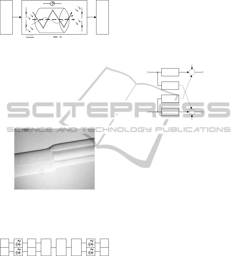
2 OPTICAL MIMO SYSTEM

MODEL

The principle of optical MIMO is based on the activa-

tion of different modes or mode groups respectively,

as illustrated in Fig. 1. In order to realize a parallel

data transmission different data sources make use of

these mode groups. A possible solution is the excita-

tion of low order mode (LOM) and high order mode

(HOM) groups. These different modes travel together

in a MMF and can be separated by their spatial distri-

bution at the receiver side leading to a (2× 2) MIMO

system in this contribution.

The excitation of the different modes can be done

through various methods. Besides using Spatial Light

Modulators (SLM) (Gu et al., 2013), Long-Period

Köhnke H., Schwinkendorf R., Daase S., Ahrens A. and Lochmann S..

Receiver Design for an Optical MIMO Testbed.

DOI: 10.5220/0005019500310036

In Proceedings of the 5th International Conference on Optical Communication Systems (OPTICS-2014), pages 31-36

ISBN: 978-989-758-044-4

 2014 SCITEPRESS (Science and Technology Publications, Lda.)

Data Source

Receiver

HOM LOM

Figure 1: Optical MIMO system by activating LOM and

HOM groups.

Gratings (LPG) (Giles et al., 2012) or Photonic Crys-

tals (Amphawan and Al Samman, 2013), the excita-

tion can simply be carried out by a centric or an eccen-

tric splice between a single-mode ﬁbre (SMF) and a

MMF. Fig. 2 illustrates a typical eccentric splice used

to excite HOM groups. Unfortunately, two SMFs’

can’t easily be placed in front of standard MMF.

That’s why other solutions are in the focus of interest.

Investigations in (Ahrens and Lochmann, 2013) have

shown that fusion couplers are capable of combining

different mode groups into a MMF.

Figure 2: Eccentric single to multi-mode ﬁbre splice (ec-

centricity 20 µm).

For mode separation at the receiver side fusion

couplers similar to the transmitter side are used. The

structure of the corresponding practical testbed is

shown in Fig. 3.

LOM

HOM

CH1

CH2

optical

coupler

optical

coupler

optical

channel

Figure 3: Structure of the optical (2× 2) MIMO testbed.

Two independent data sources (D1, D2) realized

by an Agilent high-speed pattern generator N4903B

produce unipolar signals, which drive the respective

laser diode modules with a pulse frequency of f

625 Mbit/s. The laser diodes can either work at 1326

nm or 1576 nm. Their light is fed to the centric

and eccentric splice with different power. The laser

diode, which has the higher power is used for activat-

ing the HOM, to compensate for the losses of higher

modes. Thereafter they are combined by the fusion

coupler. After the ﬁbre length of 1.9 km, the trans-

mitted signals are separated by the second fusion cou-

pler followed by two broadband Agilent 81495A re-

ceivers. The obtained signals are sampled by a high-

speed sampling oscilloscope (Agilent DSO90804A)

and stored for further off-line signal processing (CH1,

CH2). Fig. 4 shows the corresponding electrical

MIMO system model.

(t)

s 1

(t)

s 2

(t)

k 1

(t)

k 2

(t)

Figure 4: (2× 2) MIMO system model.

The n

transmit signals u

sµ

(t) (for µ = 1,.. .,n

)

are mapped to the n

received signals u

kν

(t) (for

ν = 1,.. .,n

) by using the corresponding impulse re-

sponses g

νµ

(t). Additionally, white Gaussian noise

(t) (for ν = 1,.. .,n

) is added at the receiver side.

Mathematically, the received signals can be described

kν

(t) =

∑

µ=1

sµ

(t) ∗ g

νµ

(t) + n

(t) . (1)

In this paper the number of transmitters and receivers

is limited to n

= n

= 2. The setup of the practical

(2× 2) MIMO system is shown Fig. 5.

Fig. 6 shows the measured impulse responses of

all underlying channels of this (2× 2) MIMO system

(Ahrens and Lochmann, 2013). From Fig. 6 it can

bee seen by comparing the impulse responses g

(t)

and g

(t) that the mode groups can be separated ef-

ﬁciently. Moreover, a typical high cross talk can be

identiﬁed from g

(t) and g

(t).

3 OFF-LINE SIGNAL

PROCESSING

In the following the off-line signal processing is de-

scribed including symbol clock recovery, frame syn-

chronisation, channel estimation and equalisation.

Referring to Fig 4, the MIMO channel can be divided

into four individual SISO channels. Fig. 7 shows such

OPTICS2014-InternationalConferenceonOpticalCommunicationSystems

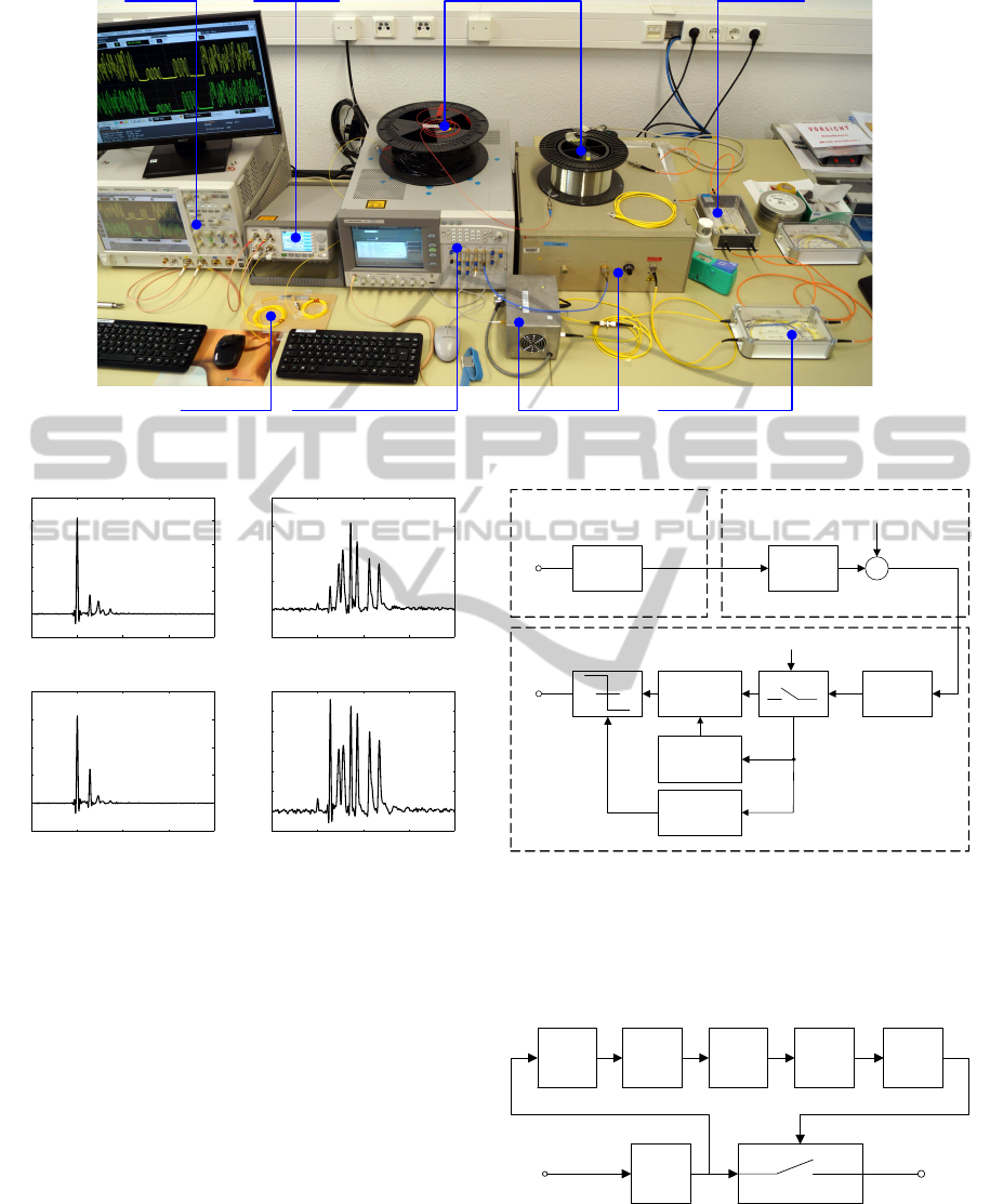
Pattern Generator (D1, D2) E/O Converter LOM/HOM Excitation

Fusion Coupler1.9 km Channel

Fusion Coupler

Oscilloscope O/E Converter

Figure 5: Setup of the practical (2× 2) MIMO system.

0 1 2 3 4

−1

0 1 2 3 4

−0.2

0.2

0.4

0.6

0.8

0 1 2 3 4

−2

0 1 2 3 4

−0.1

0.1

0.2

0.3

0.4

0.5

0.6

time (in ns) →time (in ns) →

(t) →

Figure 6: Measured MIMO speciﬁc impulse responses ap-

plying a pulse frequency of f

= 1/T

= 625 Mbit/s (ﬁbre

length of 1.9 km and diode laser wavelength 1326 nm).

a SISO channel with its corresponding off-line pro-

cessing components, which have to be combined in

case of MIMO transmission.

The starting transmitter block includes a rectan-

gular transmit ﬁlter g

(t). It is followed by the SISO

channel described by its respective impulse response.

The receiver consists of rectangular ﬁlter g

(t) and

the corresponding off-line signal processing compo-

nents.

3.1 Symbol Clock Recovery

The method of the symbol clock recovery is high-

lighted in Fig. 8. The received signals u

kν

(t) of both

MIMO-channels (i.e. for ν = 1,2) have to be squared

Transmitter

Receiver

Channel

(k)

qµ

(t)

νµ

(t)

Equalizer

(t)

sµ

(t)

kν

(t)

Channel

estim.

Frame

sync.

Figure 7: SISO system model.

in order to obtain a frequency component at the sym-

bol pulse frequency. After bandpass ﬁltering with the

symbol frequency the symbol clock can be found and

the sampled received signal u

(k) is obtained.

downsampling

kν

(t)

(k)

(t)

IFFTFFT

Filter

Max(·)

(·)

Figure 8: Symbol clock recovery.

ReceiverDesignforanOpticalMIMOTestbed

3.2 Frame Synchronization and

Channel Estimation

The sampled data are the input data for frame syn-

chronization and channel estimation. The data struc-

ture of the transmitted signal is organized as fol-

lows: The payload data are packed into 1024-bit long

frames. The structure of this frame is shown in Tab. 1.

Each frame consists of 784 bit payload (R), a 52 bit

training sequence (T) and 188 zeros (0) as guard inter-

val to compensate the delay time difference. The 52

bit training sequence consists of two 26 bit long GSM

training sequences. Since the paper concentrates on

the prove of the optical MIMO concept, the length of

the given sequences isn’t in the focus of the testbed

optimization.

The balanced 26 bit training sequence, which re-

lates to GSM standard, is used for the synchroniza-

tion and the training of the adaptive equalizer. To ﬁnd

the 52 bit sequence (T) in the data stream, the cross-

correlation function between the training sequence

and the data stream is calculated. The resulting cross-

correlation peak is now used for the frame synchro-

nisation. Furthermore, it is possible to estimate the

channel coefﬁcients by the cross-correlation function

of the inner 16 bit of the 26 bit orthogonal GSM train-

ing sequence and the corresponding sequence of the

measured data.

4 EQUALISER DESIGN

The equalization of the ﬁltered and sampled receive

signals u

(k) refers to the principle of van Etten (van

Etten, 1975; van Etten, 1976), which is illustrated in

Fig. 9. Using the channel impulse responses h

νµ

(k),

which describe the mapping of the µth input to the νth

output, i. e.

νµ

(t) = g

(t) ∗ g

νµ

(t) ∗ g

(t) , (2)

the whole MIMO system can be decomposed into a

number of SISO channels. These SISO channels in-

clude the impact of the channel as well as the transmit

and receive ﬁltering. It is assumed that the h

νµ

(k) of

each SISO channel consist of L + 1 non-zero coefﬁ-

cients. Furthermore, the noise components w

(k) are

obtained after receive ﬁltering and sampling of n

(t).

In order to remove the MIMO interferences, i.e.

interferences between the different input data streams

as well as intersymbol interferences, an appropriate

equalizer has to be chosen. A possible solution was

introduced in (van Etten, 1975; van Etten, 1976) for

estimating the corresponding MIMO speciﬁc equal-

izer coefﬁcients f

νµ

(k) (with ν = 1, 2 and µ = 1, 2).

(k)

Figure 9: (2× 2) MIMO equalizer.

The equalizer is determined similar to the zero

forcing (ZF) T-spaced equalizer known from base-

band or single-carrier transmission (Bingham, 1988).

In order to describe the whole MIMO system,

(2 × 2) submatrices H

ℓ

(for ℓ = 0,. ..,L) have to be

created taking the impact of the (2 × 2) MIMO chan-

nel at the time ℓ into account, i. e. h

νµ

[ℓ]. The (2× 2)

submatrices H

ℓ

result in

ℓ



[ℓ] h

[ℓ]

[ℓ] h

[ℓ]



. (3)

Taking the L + 1 non-zero coefﬁcients of the im-

pulse responses h

νµ

(k) into account, the interferences

within the MIMO system are described by the channel

convolution matrix H, which is given by

H =







0 · · · 0

· · · 0

L−1

· · · H

0 H

· · · H

0 0 · · · H







, (4)

where 0 is a (2× 2) zero matrix.

With the knowledge of the channel matrix H a

multidimensional equalizer can be derived similar

to the T-spaced equalizer known from the baseband

transmission. At ﬁrst a 2-dimensional Nyquist vector

z = (0...0 I 0. ..0) (5)

is deﬁned, where 0 is a (2 × 2) zero matrix and I de-

notes a (2× 2) identity matrix. The equalizer is given

according to

F =



· H



−1

· H

· z

(6)

The position of the (2× 2) identity matrix I within the

matrix z is a degree of freedom to adapt the equalizer

OPTICS2014-InternationalConferenceonOpticalCommunicationSystems

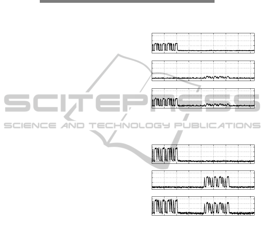
Table 1: Frame structure consisting of training sequences (T), guard intervals (0) and data (R).

D1 (LOM) T T 0 0 0 0 0 0 R 0

D2 (HOM) 0 0 0 0 T T 0 0 R 0

bit 26 26 26 26 26 26 26 26 784 32

←− 1024bit −→

to the channel conditions. Now the equalizer matrix

F can be rewritten as

F =





(7)

and the decomposition of the µth column e

provides

the equalizer impulse response f

νµ

(k), which connect

the µth (µ = 1, 2) receive ﬁlter output to the νth equal-

izer output (ν = 1,2). With the proposedZF equalizer,

the MIMO inherent interferences are removed at the

cost of an increased noise power at the detector input.

5 RESULTS

In this contribution, the channel measurements are

carried out within a 1.9 km (2 × 2) MIMO system.

For this, the HOM groups were excited by an eccen-

tricity of 15 µm. Fig. 10 and Fig. 11 illustrate the

combination of each MIMO signal u

kν

(t) by superpo-

sition of the SISO channels u

kνµ

(t).

Taking (1) into account, the MIMO signal at the

output ν (for ν = 1,2) is obtained as

kν

(t) = u

kν1

(t) + u

kν2

(t) + n

(t) . (8)

Therein the received signals u

kν1

(t) and u

kν2

(t) de-

scribe the inﬂuence of the transmitter 1 and 2, respec-

tively. Furthermore, there is a time delay between

the respective transmitted training sequence and the

crosstalk, caused by a different ﬁber length between

source and coupler of each input, which has been

compensated by the frame synchronisation module.

Based on the measured receive signals u

kν

(t) the

channel coefﬁcients h

νµ

(k) can be estimated, which

is shown in Fig. 12. With the estimated channel co-

efﬁcients the time-dispersive nature of the underly-

ing transmission channel is visible. After estimating

the channel coefﬁcients h

νµ

(k), the multidimensional

equalizer can be formed in order to remove the inter-

ferences from the MIMO system. The corresponding

eye-diagram is shown in Fig. 13 for the equalized sig-

nal u

(t).

0.02

0.04

0.06

0.02

0.04

0.06

0 25 50 75 100 125 150 175 200

0.02

0.04

0.06

k1 1

(t) (inV)

k1 2

(t) (inV)

t/T

→

Figure 10: Measured received signal u

(t) within the (2×

2) MIMO system with respect to the pulse frequency f

1/T

= 625 assuming a ﬁbre length 1.9 km.

0.02

0.04

0.06

0.02

0.04

0.06

0 25 50 75 100 125 150 175 200

0.02

0.04

0.06

k2 1

(t) (inV)u

k2 2

(t) (inV)u

(t) (inV)

t/T

→

Figure 11: Measured received signal u

(t) within the (2×

2) MIMO system with respect to the pulse frequency f

1/T

= 625 MHz assuming a ﬁbre length 1.9 km.

6 CONCLUSION

In this contribution a successful receiver design for a

(2× 2) optical MIMO system was presented. The re-

ceiver consisting of the following components: frame

synchronisation, symbol clock recovery, channel esti-

mator and equalizer was applied to a 1.9 km MIMO

testbed. The successful implementation of the MIMO

receiver was demonstrated by the open eye-diagram.

ReceiverDesignforanOpticalMIMOTestbed

−3 −2 −1 0 1 2 3

0.01

0.02

0.03

0.04

−3 −2 −1 0 1 2 3

0.001

0.002

0.003

0.004

−3 −2 −1 0 1 2 3

0.01

0.02

0.03

0.04

−3 −2 −1 0 1 2 3

0.01

0.02

0.03

0.04

(k) →

k →k →

Figure 12: Estimated channel coefﬁcients of the measured

(2× 2) MIMO signal assuming a pulse frequency of f

1/T

= 625 MHz and a ﬁbre length 1.9 km .

−0.5 −0.4 −0.3 −0.2 −0.1 0 0.1 0.2 0.3 0.4 0.5

−0.4

−0.2

0.2

0.4

0.6

0.8

1.2

1.4

t/T

(t) (inV)

Figure 13: Eye-diagram of received signal u

(t) after

equalization.

ACKNOWLEDGEMENTS

This work has been funded by the German Ministry

of Education and Research (No. 03FH016PX3).

REFERENCES

Ahrens, A. and Lochmann, S. (2013). Optical Couplers in

Multimode MIMO Transmission Systems: Measure-

ment Results and Performance Analysis. In Interna-

tional Conference on Optical Communication Systems

(OPTICS), pages 398–403, Reykjavik (Iceland).

Amphawan, A. and Al Samman, N. M. A. (2013). Tiering

Effect of Solid-Core Photonic Crystal Fiber on con-

trolled Coupling into Multimode Fiber. In Photonic

Fiber and Crystal Devices: Advances in Materials

and Innovations in Device Applications (SPIE 8847),

pages 88470Y–88470Y–6.

Bingham, J. A. C. (1988). The Theory and Practice of Mo-

dem Design. Wiley, New York.

Franz, B. and Blow, H. (2012). Experimental Evaluation of

Principal Mode Groups as High-Speed Transmission

Channels in Spatial Multiplex Systems. IEEE Pho-

tonics Technology Letters, 24:1363–1365.

Giles, I., Obeysekara, A., C., R., Giles, D., Poletti, F., and

Richardson, D. (2012). All Fiber Components for

Multimode SDM Systems. In IEEE Summer Topical

2012: Space Division Multiplexing for optical Sys-

tems and Networks, pages 212–213.

Gu, R., IP, E., Li, M. J., Huang, Y. K., and Kahn, J. M.

(2013). Experimental Demonstration of a Spatial

Light Modulator Few-Mode Fiber Switch for Space-

Division Multiplexing. In Frontiers in Optics.

K¨uhn, V. (2006). Wireless Communications over MIMO

Channels – Applications to CDMA and Multiple An-

tenna Systems. Wiley, Chichester.

Richardson, D. J., Fini, J., and Nelson, L. (2013). Space

Division Multiplexing in Optical Fibres. Nature Pho-

tonics, 7:354–362.

Sandmann, A., Ahrens, A., and Lochmann, S. (2014a).

Equalisation of Measured Optical MIMO Channels.

In International Conference on Optical Communica-

tion Systems (OPTICS), Vienna (Austria).

Sandmann, A., Ahrens, A., and Lochmann, S. (2014b). Ex-

perimental Description of Multimode MIMO Chan-

nels utilizing Optical Couplers. In 15. ITG-

Fachtagung Photonische Netze, Leipzig (Germany).

Singer, A. C., Shanbhag, N. R., and Bae, H.-M. (2008).

Electronic Dispersion Compensation– An Overwiew

of Optical Communications Systems. IEEE Signal

Processing Magazine, 25(6):110–130.

Tse, D. and Viswanath, P. (2005). Fundamentals of Wireless

Communication. Cambridge, New York.

van Etten, W. (1975). An Optimum Linear Receiver

for Multiple Channel Digital Transmission Systems.

IEEE Transactions on Communications, 23(8):828–

834.

van Etten, W. (1976). Maximum Likelihood Receiver for

Multiple Channel Transmission Systems. IEEE Trans-

actions on Communications, 24(2):276–283.

Winzer, P. (2012). Optical Networking beyond WDM.

IEEE Photonics Journal, 4:647–651.

OPTICS2014-InternationalConferenceonOpticalCommunicationSystems