Adaptive Strategies for Collaborative Work with Scale Quad-rotors
Jos´e Ces´areo Raim´undez and Jos´e Luis Cama˜no
Departamento de Ingenier´ıa de Sistemas y Autom´atica, Universidad de Vigo, Vigo, Spain
Keywords:
Collaborative Work, Adaptive Control, Quad-rotor.
Abstract:
The purpose of this paper is to present strategies for the control of movement of rigid bodies via force ac-
tuators, possibly redundant. After a nonlinear feedback linealization of the considered dynamic models and
the application of a suitable controller, an adaptive neural network based control component is incorporated
in order to cope with modeling errors and disturbance rejection. An online sequential quadratic programing
optimization with equality and inequality constraints assures an adequate configuration of actuator forces. Ap-
plication to collaborative work in the transportation of a rigid body using a squadron of scale quad-rotors is
studied.
1 INTRODUCTION
In collaborative work between different agents con-
cerning dynamic processes of mechanical nature,
such as the problem of air transport of rigid bodies,
arises the need to allocate adequate efforts to main-
tain a path and pose previously established. In this
paper this idea is applied to the collaborative work
in carrying a rigid load along a given path (Sreenath
et al., 2013) (Lee et al., 2013), using a squadron of
scale quad-rotors.
The hierarchical process of collaborative assign-
ments is shown. First, the problem of tracking a path
and pose is solved for a rigid body, which is the load
to be transported. Secondly, through an allocation
procedure based on nonlinear programming, the ef-
forts to apply at local mooring in the body transport
are determined. Finally, the determination of the or-
bits of transport agents should follow, as well as the
efforts to which they are subjected by the mooring
links with the transported body. Scale quad-rotors are
capable of aggressive maneouvering, as can be seen
in (Huang et al., 2009), (Mellinger et al., 2012). In
this last stage arises the need for adaptive augmenta-
tion, to overcome deficiencies encountered during the
modeling process or due to changing environmental
conditions.
The structure of this paper is as follows: Sec-
tion 2 introduces the development of the equations of
motion of the rigid body. In Section 3 follows the
rigid body tracking control formulation. Section 4
focuses the allocation of forces attached to the moo-
ring of the rigid body. The force allocation is formu-
lated as a nonlinear programming problem. Section
5 presents the quad-rotor simplified modeling accor-
ding to a lagrangian formulation. The quad-rotor path
error tracking controller is developed along the Sec-
tion 6 and the simulations carried out with a platoon
of quad-rotors are brought in Section 7. Finally the
conclusions are presented in Section 8. We have also
included a small appendix on the method of feedback
linearization as an introduction to the chosen control
technique.
2 RIGID BODY DYNAMICS
For the rigid body subjected to external forces, the
resulting movement equations can be described deve-
loping the Lagrangian:
T =
1
2
m
˙
ξ
⊤
˙
ξ+
1
2
ω
⊤
Jω
V = mgz
ω = Q(η)
˙
η
J
η
= Q(η)
⊤
JQ(η)
(1)
Also
˜
ω =


0 −ω
z
ω
y
ω
z
0 −ω
x
−ω
y
ω
x
0


= R(η)
˙
R
⊤
(η) (2)
319
Raimúndez J. and Camaño J..
Adaptive Strategies for Collaborative Work with Scale Quad-rotors.
DOI: 10.5220/0005017603190326
In Proceedings of the 11th International Conference on Informatics in Control, Automation and Robotics (ICINCO-2014), pages 319-326
ISBN: 978-989-758-040-6
Copyright
c
 2014 SCITEPRESS (Science and Technology Publications, Lda.)

Q(η) =


c
θ
c
ψ
−s
ψ
0
c
θ
s
ψ
c
ψ
0
−s
θ
0 1


R(η) =


c
θ
c
ψ
c
θ
s
ψ
−s
θ
c
ψ
s
θ
s
φ
−s
ψ
c
φ
s
ψ
s
θ
s
φ
+ c
ψ
c
φ
c
θ
s
φ
c
ψ
s
θ
c
φ
+ s
ψ
s
φ
s
ψ
s
θ
c
φ
−c
ψ
s
φ
c
θ
c
φ


(3)
Here m denotes the rigid body mass. ξ and ω are
the position and angular velocity in global inertial co-
ordinates and body coordinates, respectively. η are
the Euler angles pitch φ, roll θ and yaw ψ. R(η) is
the transformation matrix representing the rigid body
pose and c
θ
,s
θ
stand for cos(θ),sin(θ), etc. The iner-
tia matrix is
J =


J
1
J
12
J
13
J
12
J
2
J
23
J
13
J
23
J
3


(4)
The resulting movement equations are
¨
ξ = m
−1
( f
0
+ f)
¨
η = J
−1
η

1
2
∂
∂η
(
˙
η
⊤
J
η
˙
η) −
˙
J
η
˙
η+ τ

(5)
with f
0
= (0,0,−mg)
⊤
and f, τ the external control
forces and torques respectively.
3 RIGID BODY TRACKING
CONTROL
Given a path immersed in R
6
and named as {ξ
r
, η
r
},
define the tracking error as:
e = {e
ξ
,e
η
}
e
ξ
= ξ
r
−ξ
e
η
= η
r
−η
(6)
Imposing now a stable dynamics for the error,
¨e
ξ
+ k
ξ
d
˙e
ξ
+ k
ξ
p
e
ξ
= 0
¨e
η
+ k
η
d
˙e
η
+ k
η
p
e
η
= 0
(7)
calling {ν
ξ
, ν
η
} pseudo-controls, (5) is reduced to a
double integrator dynamics
¨
ξ = ν
ξ
¨
η = ν
η
(8)
Solving now (7) regarding {ν
ξ
, ν
η
},
ν
ξ
=
¨
ξ
r
+ k
ξ
d
˙e
ξ
+ k
ξ
p
e
ξ
= m
−1
f
0
+ m
−1
f
ν
η
=
¨
η
r
+ k
η
d
˙e
η
+ k
η
p
e
η
= J
−1
η

1
2
∂
∂η
(
˙
η
⊤
J
η
˙
η) −
˙
J
η
˙
η+ τ

(9)
From (9) we obtain the controls that keep path and
pose tracking. These controls are denoted as {f, τ}.
4 FORCE DISTRIBUTION ON
THE TIE POINTS
Consider now a set of points p
i
, i = 1,··· , n
p
given in
rigid body coordinates, just where moorings are an-
chored. Let be F
i
, i = 1,··· ,n
p
the mooring forces.
The mooring forces F
i
must be contained in a viable
subspace of its space configuration. For example,
in case that the clamping is performed by a platoon
of quad-rotors, which is the chosen setup in this pa-
per, these forces should be directed to the upper re-
gion of the geometric space in relation to the horizon-
tal plane. The forces will point to the configuration
platoon. The determination of each mooring force
F
i
, i = 1,··· ,n
p
is focused as follows, where a ∧b is
a vector product and < a, b > is a scalar product:
1. A set of equality relations g
E
concerning the ef-
forts needed to control the rigid body.
g
E
:=











f =
n
p
∑
i=1
F
i
τ =
n
p
∑
i=1
(R(η)p
i
) ∧F
i
(10)
2. The following relationship guarantees a conical
opening concerning the mooring forces. It is es-
tablished as a condition of no intersection between
the sphere |P−P
0
| = r and the line
P = p
i
+ λ
F
i
|F
i
|
, 0 < λ < ∞ (11)
such that P
0
= r
o
e
3
g
I
1
:= < R(η)p
i
−r
o
e
3
,F
i
>
2
≤ |F
i
|
2
(|R(η)p
i
−r
o
e
3
|
2
−r
2
)
, i = 1, ··· ,n
p
(12)
where e
3
= (0,0,1)
⊤
. Also r
o
, r are parameters
governing the cone aperture (see figure 1).
3. The constraints
g
I
2
:= < F
i
,e
3
> ≥0, {i = 1,...,n
p
} (13)
are needed for aperture regularization.
4. The objective function to be minimized is
F =
n
p
∑
i=1
kF
i
k (14)
ICINCO2014-11thInternationalConferenceonInformaticsinControl,AutomationandRobotics
320

The nonlinear optimization problem can be for-
mulated as:
Minimize F(X) such that
X ∈ {g
E
(X) ∩g
I
1
(X) ∩g
I
2
(X)}
(15)
The process of minimization is fast and efficient
using a minimization method such as the Sequen-
tial Quadratic Programming Method (Nocedal and
Wright, 1999). The initial point at each sample time is
the solution previously found at the previous sample
time.
Once determined the forces, the cabled ties are
propagated in the corresponding direction to a desired
length l
i
, at which point the respective quad-rotor will
absorb the effort. Thus, the position reference trajec-
tory of the quad-rotors is obtained by:
ξ
i
r
= R(η)p
i
+ ξ + l
i
F
i
|F
i
|
, i = 1,··· ,n
p
(16)
p
1
p
2
p
3
p
4
F
1
F
2
F
3
F
4
r
o
r
Figure 1: Auxiliary sphere in the definition of feasible lift-
ing forces.
5 QUAD-ROTOR: SIMPLIFIED
MODELING AND
LAGRANGIAN FORMULATION
The generalized coordinates for a quad-rotor are q =
(ξ
q
,η
q
) where ξ
q
= (x
q
,y
q
,z
q
), denote the position
of the center of mass concerning the inertial frame
and η
q
= (ψ
q
,θ
q
,φ
q
) are the three Euler angles (yaw,
pitch and roll) representing the quad-rotor pose. The
total quad-rotor kinetic energy is given by T
q
and the
potential energy is given by V
q
with the corresponding
lagrangian L
q
= T
q
−V
q
(Avila-Vilchis et al., 2003)
(Koo et al., 2001), with
T
q
=
1
2
m
q
˙
ξ
⊤
q
˙
ξ
q
+
1
2
ω
⊤
q
J
q
ω
q
V
q
= m
q
gz
q
ω
q
= Q(η
q
)
˙
η
q
(17)
Here m
q
denotes the mass of the quad-rotor and
R(η
q
), Q(η
q
) are defined in (3). The quad-rotor iner-
tia matrix is given by
J
q
=


J
q
1
J
q
12
J
q
13
J
q
12
J
q
2
J
q
23
J
q
13
J
q
23
J
q
3


J
η
q
= Q(η
q
)
⊤
J
q
Q(η
q
)
(18)
Here J
η
q
is the inertia matrix regarding the inertial
frame. The movement equations are:
¨
ξ
q
= −m
−1
q
( f
0
−F
i
+ R(η
q
) f
b
)
¨
η
q
= J
−1
η
q
(η
q
)

1
2
∂
∂η
q

˙
η
⊤
q
J
η
q
˙
η
q

−
˙
J
η
q
˙
η
q
+ R(η
q
)τ
η
q
i
(19)
with
f
b
=


0
0
u


, f
0
=


0
0
−m
q
g


(20)
and τ
η
q
= (τ
ψ
q
,τ
θ
q
,τ
φ
q
) being the moments regarding
the body frame. Those moments can be modeled in a
first degree of approximation, and in the local frame
without considering rotor dynamics, as:
u =
4
∑
j=1
f
j
f
j
= B
o
ω
2
j
τ
ψ
q
= (D
o
/B
o
)( f
2
+ f
4
− f
1
− f
3
)
τ
θ
q
= l( f
4
− f
2
)
τ
φ
q
= l( f
3
− f
1
)
(21)
where f
j
are the lifting forces in each rotor, ω
j
the corresponding angular velocities, l the diagonal
distance between axes of the respective rotors, and
D
o
, B
o
are drag and thrust factors, respectively. The
relationship between {f
b
, τ
η
q
} and rotations ω
j
is:
ω
2
1
=
1
4B
o
D
o
l
(D
o
lu −2D
o
τ
φ
q
−B
o
lτ
ψ
q
)
ω
2
2
=
1
4B
o
D
o
l
(D
o
lu −2D
o
τ
θ
q
+ B
o
lτ
ψ
q
)
ω
2
3
=
1
4B
o
D
o
l
(D
o
lu + 2D
o
τ
φ
q
−B
o
lτ
ψ
q
)
ω
2
4
=
1
4B
o
D
o
l
(D
o
lu + 2D
o
τ
θ
q
+ B
o
lτ
ψ
q
)
(22)
6 QUAD-ROTOR ERROR
TRACKING CONTROLLER
Each quad-rotor will assume the controller role at
each mooring link. Each quad-rotor must provide
AdaptiveStrategiesforCollaborativeWorkwithScaleQuad-rotors
321

enough effort to counterbalance the mooring force F
i
,
while maintaining the required path defined through
(16). Ideally the link to establish will read ξ
i
r
= ξ
i
q
where ξ
i
r
are the reference position of the center of
gravity of the i-th quadrotor and are given by (16)
(theoretical anchor point). Instead we will impose a
stable error dynamics criteria such as
¨e
i
+ K
d
˙e
i
+ K
p
e
i
= 0 {K
d
≻ 0, K
p
≻ 0} (23)
in which
e
i
= (e
i
ξ
, e
i
η
) = P
i
r
−P
i
q
(24)
with
P
i
r
= (ξ
i
r
, η
i
r
)
P
i
q
= (ξ
i
q
, η
i
q
)
(25)
the reference and actual trajectories of the i-th quadro-
tor. Establishing now
¨e
i
ξ
=
¨
ξ
i
r
+ m
−1
q
( f
0
−F
i
) + m
−1
q
R(η
i
q
) f
i
b
= ν
i
ξ
= −k
pξ
e
i
ξ
−k
dξ
˙e
i
ξ
¨e
i
η
=
¨
η
i
r
−J
−1
η
i
q
"
1
2
∂
∂η
i
q

˙
η
i⊤
q
J
η
i
q
˙
η
i
q

−
˙
J
η
i
q
˙
η
i
q
+ R(η
i
q
)τ
i
q
i
= ν
i
η
= −k
pη
e
i
η
−k
dη
˙e
i
η
(26)
with (ν
i
ξ
, ν
i
η
) the pseudo-control components and k
pξ
,
k
pη
, k
dξ
, k
dη
positive matrices. Here F
i
is the mooring
force attached to the i-th quad-rotor. The expression
for ¨e
i
is obtained substituting (19) in (23). From
¨
ξ
i
r
+ m
−1
q
( f
0
−F
i
) + m
−1
q
R(η
i
o
) f
i
b
= ν
i
ξ
(27)
with f
i
b
= u
i
e
3
and solving for {u
i
, θ
i
o
, φ
i
o
} the system
of equations
R(η
i
o
) f
i
b
= Φ
i
= m
q
(ν
i
ξ
−
¨
ξ
i
r
) + F
i
− f
0
(28)
we obtain
η
i
o
=





θ
i
o
= arctan

q
Φ
i
y
2
+ Φ
i
z
2
, Φ
i
x

φ
i
o
= arctan

−Φ
i
z
, −Φ
i
y

u
i
=


Φ
i


(29)
where η
i
o
is the needed attitude. Calling now as atti-
tude correction
∆η
i
:=


0
θ
i
r
−θ
i
o
φ
i
r
−φ
i
o


(30)
and including the attitude correction in the attitude er-
ror dynamics, results in
ν
i
η
= −k
pη
(e
i
η
−∆η
i
) −k
dη
˙e
i
η
(31)
which defines the control law:
τ
i
=
˙
J
η
i
q
˙
η
i
q
−
1
2
∂
∂η
i
q

˙
η
i⊤
q
J
η
i
q
˙
η
i
q

+ J
η
i
q

¨
η
i
r
+ k
pη
(e
i
η
−∆η
i
) + k
dη
˙e
i
η

(32)
This control will stabilize the P
i
r
trajectory tracking
with a bounded error. In figure 2 the structure of the
controller is shown, consisting of two proportional-
derivative terms, namely PD
ξ
, PD
η
where S
ξ
, S
η
re-
present the operations described in equations (27)
and (32) respectively. QR represents the plant (quad-
rotor) and C the generator of trajectory commands.
6.1 Adaptive Augmentation
In order to cancel the presence of unmodeled dynam-
ics, two corrective components are added to the con-
trol loops presented in figure 2, which are generated
by the single hidden layer neural network adaptive el-
ement defined by SHL-NN = (NN
ξ
, NN
η
). In what
follows the control of each quadrotor is analyzed and
the superindex i for the i-th quad-rotor is omitted for
the sake of clarity. Also the q subindex is omited in
ξ
q
, η
q
.
Let ∆ = (∆
ξ
, ∆
η
) be the vector of modeling errors.
Equations (26) can be written as:
¨e
ξ
=
¨
ξ
r
−(
¨
ξ+ ∆
ξ
)
¨e
η
=
¨
η
r
−(
¨
η+ ∆
η
)
(33)
By adding to the control effort the adaptive terms
ν
aξ
, ν
aη
the following representation of the error dy-
namics is obtained:
¨e
ξ
+ k
pξ
e
ξ
+ k
dξ
˙e
ξ
+ ν
aξ
−∆
ξ
= 0
¨e
η
+ k
pη
e
η
+ k
dη
˙e
η
+ ν
aη
−∆
η
= 0
(34)
which can also be written as
d
dt

e
˙e

=

O I
−K
p
−K
d

e
˙e

+ B(ν
a
−∆)
(35)
with
K
p
=

k
pξ
O
O k
pη

, K
d
=

k
dξ
O
O k
dη

B =

O
I

, ν
a
=

ν
aξ
ν
aη

, ∆ =

∆
ξ
∆
η

(36)
and with e = (e
ξ
, e
η
). Here again, O, I are suitable
null and identity matrices respectively. If the SHL-
NN output signal ν
a
perfectly cancels ∆, then we
ICINCO2014-11thInternationalConferenceonInformaticsinControl,AutomationandRobotics
322

C
¨η
r
¨
ξ
r
u
∆η
η
r
, ˙η
r
P D
ξ
S
ξ
P D
η
S
η
τ
η
ξ,
˙
ξ
ξ
r
,
˙
ξ
r
η, ˙η
QR
NN
ν
aξ
ν
aη
Figure 2: Augmented Linear Controller with an Adaptive SHL-NN.
have asymptotically stable error dynamics. ν
a
has the
structure
ν
a
=

W
⊤
ξ
¯
σ(V
⊤
ξ
¯
ξ),W
⊤
η
¯
σ(V
⊤
η
¯
η)

(37)
Weight propagation for W
{ξ,η}
,V
{ξ,η}
is done accor-
ding to the adaptation laws
˙
W
i
= −[(
¯
σ−
¯
σ
′
V
⊤
i
¯q)r
⊤
+ κkekW
i
]Γ
W
i
˙
V
i
= −Γ
V
i
[ ¯q(r
⊤
W
⊤
i
¯
σ
′
) + κkekV
i
]
(38)
with r = (e
⊤
PB)
⊤
, and i= {ξ, η}. The representation
of
¯
σ(V
⊤
ξ
¯q) as
¯
σ, as well as that of
¯
σ
′
, is done for the
sake of clarity. Γ
V
i
≻ 0, Γ
W
i
≻ 0 are definite positive
matrices and κ > 0 is a real constant, being ¯q the ex-
tended input vector, that is, ¯q = (1, q) where q is the
input vector.
6.2 Obtaining the Adaptation Laws
Let us consider the Lyapunov function
V(e,
˜
V,
˜
W) =
1
2

e
⊤
Pe
+tr

˜
W
⊤
Γ
−1
W
˜
W

+ tr

˜
V
⊤
Γ
−1
V
˜
V

(39)
where P solves the equation
A
⊤
P+ PA+ Q = 0, A =

O I
−K
p
−K
d

(40)
with −Q and P definite positive. In order to obtain the
adaptation equations (38) we must follow the steps re-
quired to proof that, on the error orbits, the condition
˙
V ≤ 0 is satisfied as explained in (Kannan and John-
son, 2002). The following steps are given in order
to show the parameters regarding an adequate tuning
of the controller. The details of the proof of conver-
gence follow the above mentioned reference. Let us
consider
ε = ν
∗
a
−∆ = W
∗⊤
¯
σ(V
∗⊤
¯q) −∆ (41)
where W
∗
, V
∗
are the optimum values that best ap-
proximate ∆. The error dynamics is
˙e = Ae + B

W
∗⊤
¯
σ(V
⊤
¯q) −W
⊤
¯
σ(V
∗⊤
¯q) + ε

(42)
Defining now
˜
W = W −W
∗
,
˜
V = V −V
∗
and using
the Taylor series expansion of σ with respect to V in
the neighborhood of V
∗
, which is the optimum value,
we obtain
˙e = Ae+ B

˜
W
⊤
(σ−σ
′
V
⊤
¯q) + W
⊤
σ
′
˜
V
⊤
¯q+ w

(43)
with
w = ε−W
∗⊤

σ
∗
−σ+ σ
′
˜
V
⊤
¯q

+
˜
W
⊤
σ
′
V
∗⊤
¯q (44)
Substituting now (38) and (43) in the expression of
˙
V
we have
˙
V = −
1
2
e
⊤
Qe+ e
⊤
PBw−κkektr

˜
Z
⊤
Z

(45)
where
Z =

V 0
0 W

,
˜
Z = Z −Z
∗
(46)
Using tr(
˜
Z
⊤
Z) ≤


˜
Z


kZ
∗
k −


˜
Z


2
and following
(Kannan and Johnson, 2002) there exist a
0
,a
1
,c
3
,κ >
kPBkc
3
such that
˙
V =−
1
2
λ
min
(Q)kek
2
−(κ −kPBkc
3
)kek


˜
Z


2
+ a
0
kek+ a
1
kek


˜
Z


(47)
and, with Z
m
=
a
1
+
√
a
2
1
+4a
0
(κ−kPBkc
3
)
κ−kPBkc
3
,
kek ≥
a
0
+ a
1
Z
m
1
2
λ
min
(Q)
⇒
˙
V ≤0 (48)
Thus for convenient initial conditions, the tracking e-
rror e is ultimately uniformly bounded.
AdaptiveStrategiesforCollaborativeWorkwithScaleQuad-rotors
323

7 SIMULATION RESULTS
In this section we perform the simulation of a ty-pical
maneuver, in which a rigid body is transported in an
upward helical path, using four identical quad-rotors
on the task. During transport the body and the quad-
rotors suffer the action of an intense wind gust along
the x,y,z axes modeled by
f
x
= ρ
x
exp

t −t
x
σ
x

2
!
f
y
= ρ
y
exp

t −t
y
σ
y

2
!
f
z
= ρ
z
exp

t −t
z
σ
z

2
!
(49)
where ρ
x
= ρ
y
= ρ
z
= 2, t
x
= 25, t
y
= 35, t
z
=
40, σ
x
= σ
y
= σ
z
= 2. The main parametric va-
lues in this simulation are: m = 3, J
1
= 1, J
2
=
2, J
3
= 4, the mooring points in body coordi-
nates p
1
= (2,1, 0.2)
⊤
, p
2
= (2,−1,0.2)
⊤
, p
3
=
(−2,−1, 0.2)
⊤
, p
4
= (−2, 1, 0.2)
⊤
and the mooring
ropes with l
1
= l
2
= l
3
= l
4
= 20. For the restric-
tion sphere r = 3.5, r
o
= 4. The path and rigid body
pose of the load g.c. along the trip are given by P
ξ
=
(ρsin(Ωt), ρcos(Ωt),V
c
t + h
o
)
⊤
and P
η
= (0,0, Ωt)
⊤
with Ω = 0.1, V
c
= 0.1. For each quad-rotor the main
data is: m
q
= 2, J
q
1
= 0.5, J
q
2
= 0.5, J
q
3
= 0.2, k
p
ξ
=
16, k
d
ξ
= 4, k
p
η
= 120, k
d
η
= 12, γ
W
ξ
= γ
W
η
= γ
V
ξ
=
γ
V
η
= 2, κ
ξ
= κ
η
= 4.
10
20
30
40
50
60
7.2
7.6
7.8
8.0
8.2
8.4
8.6
Figure 3: Module forces |F
i
| in the four ropes during the
maneuver, including simultaneous wind gusts along the
{x,y,z} axes.
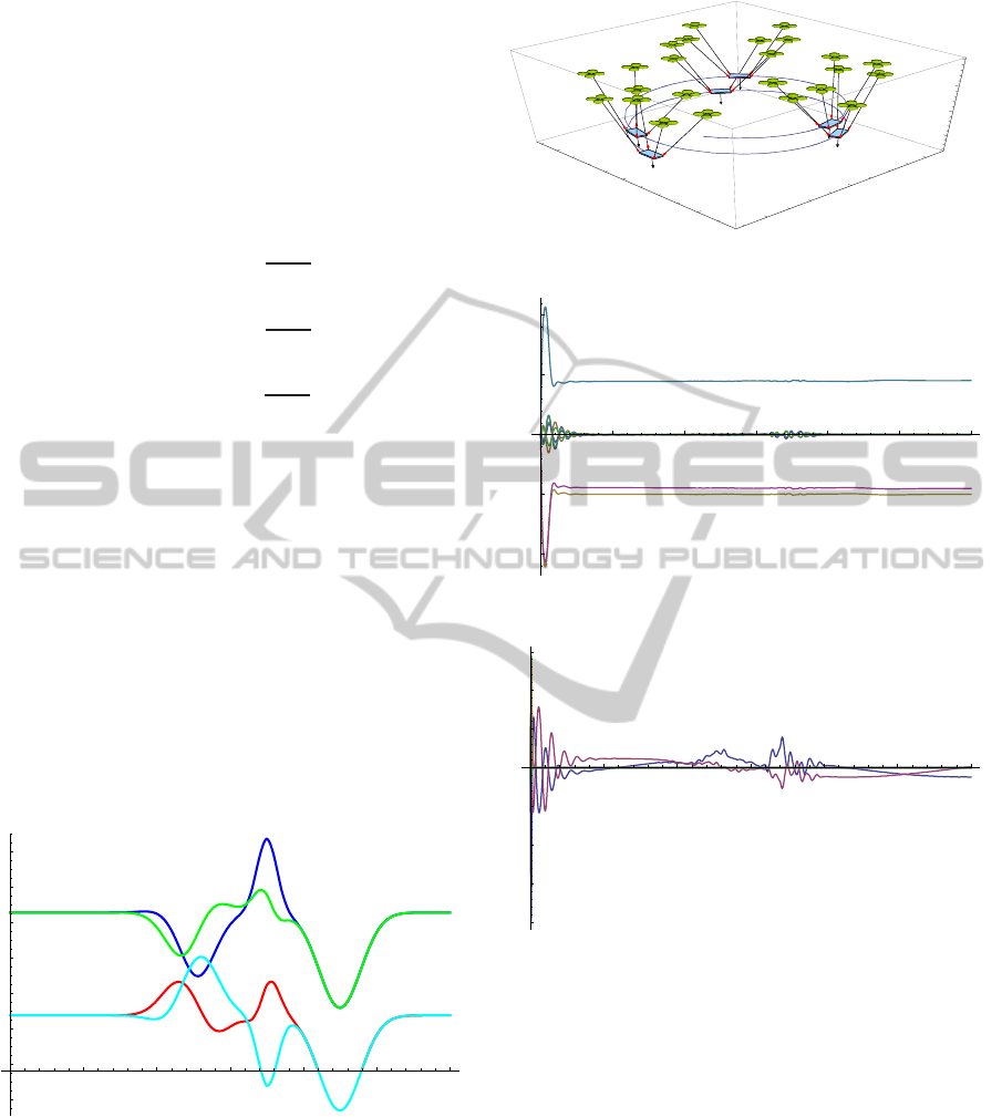
8 CONCLUSIONS
The method presented provides guidelines for the
transport of rigid loads through the collaborative ef-
fort between agents. Within this approachcan also ad-
-20
0
20
-20
0
20
0
10
20
30
Figure 4: Evolution of a transport maneuver.
10
20
30
40
50
60
-1.0
-0.5
0.5
1.0
Figure 5: Evolution of W
ξ
weights in a typical maneuver.
10
20
30
40
50
60
-4
-3
-2
-1
1
2
3
Figure 6: Evolution of W
η
weights in a typical maneuver.
dressed the problem of failures with consequent redis-
tribution of loads among agents. Substituting stable
dynamic error cancelation instead of equality holo-
nomic links, can be an effective simplification pro-
cedure, according to the simulation results.
ACKNOWLEDGEMENTS
This work was supported by the Spanish Ministry of
Science and Education, grant DPI-2010-20466-C02-
01.
ICINCO2014-11thInternationalConferenceonInformaticsinControl,AutomationandRobotics
324

REFERENCES
Avila-Vilchis, J., Brogliato, B., Dzul, A., and Lozano,
R. (2003). Nonlinear modeling and control of heli-
copters. Automatica, 39:1583–1596.
Hornik, K., Stinchcombe, M., and White, H. (1989). Multi-
layer feedforward networks are universal approxima-
tors. IEEE Transactions on Neural Networks, 2:359–
366.
Huang, H., Hoffmann, G., Waslander, S., and Tomlin, C.
(2009). Aerodynamics and control of autonomous
quadrotor helicopters in aggressive maneuvering. In
IEEE International Conference on Robotics and Au-
tomation, Japan.
Isidori, A. (1995). Nonlinear control systems. Communica-
tions and Control Engineering. Springer.
Johnson, E. (2000). Limited Authority Adaptive Flight Con-
trol. PhD thesis, Georgia Institute of Technology.
Kannan, S. and Johnson, E. (2002). Adaptive flight con-
trol for an autonomous unmanned helicopter. In AIAA
Guidance, Navigation, and Control Conference and
Exhibit, pages 1–11.
Kim, N. (2003). Improved methods in neural network based
adaptive output feedback control, with applications to
flight control. PhD thesis, Georgia Institute of Tech-
nology.
Koo, T., Ma, Y., and Sastry, S. (2001). Nonlinear control
of a helicopter based unmanned aerial vehicle model.
Technical report, UC Berkeley.
Lee, T., Sreenath, K., and Kumar, V. (2013). Geometric
control of cooperating multiple quadrotor uavs with a
suspended payload. In IEEE Conference on Decision
and Control.
Mellinger, D., Michael, N., and Kumar, V. (2012). Tra-
jectory generation and control for precise aggressive
maneuvers with quadrotors. International Journal of
Robotics Research, 31:664–674.
Nardi, F. (2000). Neural Network Based Adaptive Algo-
rithms for Nonlinear Control. PhD thesis, Georgia In-
stitute of Technology.
Nocedal, J. and Wright, S. (1999). Numerical Optimization
(Chapters 12, 18). Prentice Hall.
Shin, Y. (2005). Neural Network Based Adaptive Control
for Nonlinear Dynamic Regimes. PhD thesis, Georgia
Institute of Technology.
Sreenath, K., Michael, N., and Kumar, V. (2013). Trajectory
generation and control of a quadrotor with a cable-
suspended load. a differentially-flat hybrid system. In
IEEE International Conference on Robotics and Au-
tomation, pages 4888–4895.
APPENDIX
Approximate System Linearization
One common method for controlling nonlinear dy-
namical systems is based on approximate feedback
linearization (Isidori, 1995), which depends on the
relative degree of each controlled variable. For new-
tonian systems like the quad-rotor in a simplified ap-
proach, the regulated variables of interest, here repre-
sented as the vector q, have relative degree two
¨q = f(q, ˙q,u) (50)
The control variables are represented by the vector u.
A pseudo control ν is defined such that the dynamic
relation between it and the system state is linear ¨q = ν
where ν = f(q, ˙q,u). Since the function f(q, ˙q,u) is
not exactly known, an approximation ν =
ˆ
f(q, ˙q,u) is
used which is invertible regarding u, resulting in
¨q = ν+ ∆(q, ˙q,u) (51)
where the modeling error is represented by
∆(q, ˙q,u) = f(q, ˙q,u) −
ˆ
f(q, ˙q,u) (52)
So the effective actuator can be calculated as
ˆu =
ˆ
f
−1
(q, ˙q, ν) (53)
Supposing in (51) that ∆(q, ˙q, u) = 0 we can proceed
in the stabilization problem, choosing a linear con-
troller, a PD for instance, that will locally solve the
regulation problem. A single hidden layer (SHL) neu-
ral network with convenientlyadapted weights will be
responsible for modeling error cancelation. Including
a command path generator C, the former linear con-
troller can be augmented through the architecture de-
picted in figure 7.
+
-
+
+
-
C
PD
ˆ
f
−1
(q, ˙q, ν)
Plant
SHL-NN
¨q
r
ν
P D
ν
ν
a
q
r
q
ˆu
e
Figure 7: NN augmented adaptive control architecture.
The pseudo control signal in (51) is the sum of
three components
ν = ¨q
r
+ ν
PD
−ν
a
(54)
where ¨q
r
is generated by C, ν
PD
is generated by
the PD controller and ν
a
is generated by the adap-
tive element introduced to compensate for the model
inversion error. The tracking error is computed as
e = [q
r
−q, ˙q
r
− ˙q]
T
and the PD controller can be re-
presented by
ν
PD
=

K
p
K
d

e (55)
so the tracking error dynamics is given by
˙e = Ae+ B(ν
a
−∆) (56)
AdaptiveStrategiesforCollaborativeWorkwithScaleQuad-rotors
325

with
A =

O I
−K
p
−K
d

, B =

O
I

(57)
where I and O are a suitable identity and null matrices
respectively.
Adaptive Element
The adaptive element is implemented by a SHL-NN
with conveniently tuned weights V,W such that
ν
a
= W
⊤
¯
σ(V
⊤
¯q) (58)
with ¯q = [ν,q]. Given a sufficient number of hidden
layer neurons and appropriate inputs, it should be pos-
sible to train a SHL-NN (Hornik et al., 1989) on line
to cancel the effect of ∆. The weight matrices are
V =




v
0,1
v
0,2
··· v
0,n
2
v
1,1
v
1,2
··· v
1,n
2
.
.
.
.
.
.
.
.
.
.
.
.
v
n
1
,1
v
n
1
,2
··· v
n
1
,n
2




W =




w
0,1
w
0,2
··· w
0,n
3
w
1,1
w
1,2
··· w
1,n
3
.
.
.
.
.
.
.
.
.
.
.
.
w
n
2
,1
w
n
2
,2
··· w
n
2
,n
3




(59)
Here n
1
,n
2
,n
3
are the number of inputs, hid-
den layer nodes and outputs. Also
¯
σ(ξ) =
(1,σ(ξ
1
),··· , σ(ξ
n
1
))
⊤
. The scalar function σ is the
sigmoidal activation function σ(ξ) = 1/(1+ e
−αξ
).
Contractibility
The transformation ν
a
=W
⊤
¯
σ(V
⊤
¯q) must be contrac-
tive regarding ν
a
. Note that ∆ depends on ν
a
through
ν, whereas ν
a
has to be designed to cancel ∆. Hence
the existence and uniqueness of a fixed point solution
for ν
a
= ∆(q, ˙q, ν
a
) must be assumed. A sufficient
condition is to ascertain that the map ν
a
→∆(q, ˙q,ν
a
)
is a contraction over the entire input domain of inter-
est, or k∂∆/∂ν
a
k < 1. This condition is equivalent to
(Kim, 2003) (Johnson, 2000) (Kannan and Johnson,
2002)
0 <
1
2




∂f
∂u




<




∂
ˆ
f
∂u




< ∞ (60)
Consider the system (50), the inverse law ˆu =
ˆ
f
−1
(q, ˙q,ν) and the contractibility property, as well
as the adaptation laws
˙
W = −

(
¯
σ−
¯
σ
′
V
⊤
¯q)r
⊤
+ κkekW

Γ
W
˙
V = −Γ
V

¯q(r
⊤
W
⊤
¯
σ
′
) + κkekV

(61)
where
¯
σ
′
(ˆz) =
∂
¯
σ(z)
∂z



z=ˆz
is the Jacobian matrix and
r = e
⊤
PB. Also P ≻ 0 is the unique positive definite
solution for the Lyapunov equation A
⊤
P+ PA+Q = 0
for any convenient Q ≻ 0. A and B are defined in
(57). Given (61) with Γ
W
≻ 0, Γ
V
≻ 0 and κ > 0,
according to (Nardi, 2000), (Shin, 2005) the tracking
error e uniform boundedness is assured.
ICINCO2014-11thInternationalConferenceonInformaticsinControl,AutomationandRobotics
326