
Speeding up Support Vector Machines
Probabilistic versus Nearest Neighbour Methods for Condensing Training Data
Moïri Gamboni, Abhijai Garg, Oleg Grishin, Seung Man Oh, Francis Sowani,
Anthony Spalvieri-Kruse, Godfried T. Toussaint and Lingliang Zhang
Faculty of Science, New York University Abu Dhabi, P.O. Box 129188, Abu Dhabi, U.A.E.
Keywords: Machine Learning, Data Mining, Support Vector Machines, SMO, Training Data Condensation, k-nearest
Neighbour Methods, Blind Random Sampling, Guided Random Sampling, Wilson Editing, Gaussian
Condensing.
Abstract: Several methods for reducing the running time of support vector machines (SVMs) are compared in terms
of speed-up factor and classification accuracy using seven large real world datasets obtained from the UCI
Machine Learning Repository. All the methods tested are based on reducing the size of the training data that
is then fed to the SVM. Two probabilistic methods are investigated that run in linear time with respect to the
size of the training data: blind random sampling and a new method for guided random sampling (Gaussian
Condensing). These methods are compared with k-Nearest Neighbour methods for reducing the size of the
training set and for smoothing the decision boundary. For all the datasets tested blind random sampling gave
the best results for speeding up SVMs without significantly sacrificing classification accuracy.
1 INTRODUCTION
One of the most attractive learning machine models
for pattern recognition applications, from the point
of view of high classification accuracy, appears to be
the Support Vector Machine (SVM) (Vapnik, 1995).
There exists empirical evidence that SVMs yield
lower rates of misclassification than even the
classical k-Nearest Neighbour rule (Toussaint and
Berzan, 2012), in spite of the fact that (at least in
theory) the latter is asymptotically Bayes optimal for
all underlying probability distributions (Devroye,
1981). The drawback of SVMs is their worst-case
complexity, which is O(N
3
), where N is the number
of instances in the training set, so that for very large
datasets the training time may become prohibitive
(Bordes, Ertekin, Weston, Bottou, 2005.). Therefore
much effort has been devoted to finding ways to
speed up SVMs (Almeida, Braga, and Braga, 2000;
Chen and Chen, 2002; Panda, Chang, and Wu, 2006;
Wang, Zhou, Huang, Liang, and Yang, 2006; Chen
and Liu, 2011; Li, Cervantes and Yu, 2012; Liu,
Beltran, Mohanchandra and Toussaint, 2013; Chen,
Zhang, Xue, and Liu, 2013). The simplest approach
is to select a small random sample of the data for
training (Lee and Mangasarian, 2001). This
approach may be trivially implemented in O(N)
worst-case time. Here this method is called blind
random sampling because it uses no information
about the underlying structure of the data. Non-blind
random sampling techniques such as Progressive
Sampling (PS) and Guided Progressive Sampling
(GPS) have also been investigated with some
success (Provost, Jensen and Oates, 1999; Ng and
Dash, 2006; Portet, Gao, Hunter and Quiniou, 2007).
Non-random sampling methods attempt to use
intelligent data analysis such as genetic algorithms
(Kawulok and Nalepa, 2012) or proximity graphs
(Toussaint and Berzan, 2012; Liu, Beltran,
Mohanchandra and Toussaint, 2013) to preselect a
supposedly better representative subset of the
training data, which is then fed to the SVM, in lieu
of the large original set of data. However, the use of
guided data condensation methods usually incurs an
additional worst-case cost of O(N log N) to O(N
3
).
Since 1968 the literature contains a plethora of such
algorithms and heuristics of varying degrees of
computational complexity, for preselecting small
subsets of the training data that will perform well
under a variety of circumstances (Hart, 1968;
Sriperumbudur & Lanckriet, 2007; Toussaint, 2005).
Although such techniques naturally speed up the
training phase of the SVMs, by virtue of the smaller
364
Gamboni M., Garg A., Grishin O., Man Oh S., Sowani F., Spalvieri-Kruse A., T. Toussaint G. and Zhang L..
Speeding up Support Vector Machines - Probabilistic versus Nearest Neighbour Methods for Condensing Training Data.
DOI: 10.5220/0004927003640371
In Proceedings of the 3rd International Conference on Pattern Recognition Applications and Methods (ICPRAM-2014), pages 364-371
ISBN: 978-989-758-018-5
Copyright
c
2014 SCITEPRESS (Science and Technology Publications, Lda.)

size of the training data, many studies primarily
focus on and report only the number of support
vectors retained, ignoring the additional time taken
to perform the pre-selection. Indeed, it has been
shown empirically, for methods that used proximity
graphs for training data condensation, that if the
additional time taken by the pre-selection step is
taken into consideration, the overall training time is
generally much worse than that of simple blind
random sampling (Liu, Beltran, Mohanchandra and
Toussaint, 2013).
Some hybrid methods that combine blind random
sampling with structured search for good
representatives of datasets have also been tried. An
original method combining blind random sampling
with SVM and near neighbour search, has recently
been suggested by Li, Cervantes and Yu (2012).
Their approach first uses blind random sampling to
select a small subset of the data, from which the
support vectors are extracted using a preliminary
SVM. These support vectors are then used to select
points from the original training set (the data
recovery step) that are near the preliminary support
vectors, thus yielding the condensed training set on
which the final SVM is applied.
In this paper several methods for speeding up the
running time of support vector machines (SVMs) are
compared in terms of the speed-up factor and the
classification accuracy, using seven large real world
datasets taken from the University of California at
Irvine Machine Learning Repository (Bache,
Lichman, 2013). All the methods are based on
efficiently reducing the size of the training data that
is subsequently fed to the SVM (SMO). Two
probabilistic methods are investigated that run in
O(N) worst-case time. The first uses blind random
sampling and the second is a new method proposed
here for guided random sampling (Gaussian
Condensing). These methods are also compared with
the standard leading competitor, the k-Nearest
Neighbour rule, as well as nearest neighbour
methods for reducing the size of the training set (k-
NN condensing), and for smoothing the decision
boundary (Wilson editing), both of which run in
O(N
2
) worst-case time.
2 THE CLASSIFIERS TESTED
2.1 Blind Random Sampling
Blind random sampling is the simplest method for
reducing the size of the training set, both
conceptually and computationally, with a running
time of O(N). Its possible drawback, in theory, is
that it is blind with respect to the quality of the
resulting reduced training set, although this need not
result in poor performance. In the experiments
reported here the percentages of training data
randomly selected for training the SVM (SMO) were
varied from 10% to 90% in increments of 10%.
2.2 Wilson Editing (Smoothing)
Wilson’s editing algorithm was used for smoothing
the decision boundary (Wilson, 1973). Each instance
X in the training set is classified using the 3-Nearest
Neighbour rule (the three nearest neighbours of X,
not including itself). Classification is done by means
of a majority vote. If the instance is misclassified it
is marked. After all instances have been classified,
all the marked points are deleted. This condensed set
is then used to classify the testing set. Wilson editing
was not designed to significantly reduce the size of
the training set; its goal is rather to improve
classification accuracy, and is used here as a pre-
processing step before reducing the training set
further with methods tailored for that purpose. Since
k = 3, Wilson smoothing runs in O(N
2
) worst-case
time using software packages available in the Weka
Machine Learning Software (Witten and Frank,
2000), and a straightforward naïve implementation.
2.3 k-nearest-Neighbour Condensation
When all k nearest neighbours of a point X belong to
the class of X, the k-NN rule makes a decision with
very high confidence. In other words the point X is
surrounded by close data points from its own class,
and is therefore located relatively far from the
decision boundary. This suggests that many points
with this property could be safely deleted. Before
classifying each testing set, the corresponding
training set is condensed as follows. Each instance in
the training set is classified using the k-NN rule (not
including itself). If the instance is correctly
classified with very high confidence it is marked.
After all instances are classified, all marked points
are deleted. This condensed set is then used to
classify the testing set. High confidence in the
classification of X is measured by the proportion of
the k nearest neighbours of X that belong to the class
of X. The standard k-NN rule uses a majority vote as
its measure of confidence. In our approach we use
the unanimity vote (all the k nearest neighbours
belong to the same class), and select a good value of
k. This algorithm runs in O(kN
2
) worst-case time
using the naïve straightforward implementation and
SpeedingupSupportVectorMachines-ProbabilisticversusNearestNeighbourMethodsforCondensingTrainingData
365

packages available in Weka. Note that when data of
different classes are widely separated it may happen
(at least in theory) that for every point X its k nearest
neighbours all belong to the class of X. In such a
situation the unbridled k-NN condensation might
discard the entire training set. For such an
eventuality, if for some pattern class all training
instances are marked for deletion, the mean of those
instances is retained as the representative of that
class. Experiments were also performed with k-NN
condensation preceded by Wilson editing.
2.4 Gaussian Condensing
Gaussian Condensing is a novel heuristically guided
random sampling algorithm introduced here. The
heuristic implemented assumes that instances with
feature values relatively close to the mean of their
own class are likely to be furthest from the decision
boundary, and therefore not expected to contain
much discrimination information. Conversely, points
relatively far from the mean are likely to be closer to
the decision boundary, and expected to contain the
most useful information. First, for each class, the
mean value of each feature is calculated. Then, for
each feature in each instance, the ratio between the
Gaussian function of the mean, and the Gaussian
function of the feature value of that instance is
computed. This determines a parameter termed the
partial discarding probability. Finally, all instances
are discarded probabilistically in parallel with a
probability equal to the mean of the partial
discarding probabilities of all their features. The
main attractive attribute of this algorithm is that it
runs in O(N) worst-case time, where N is the number
of training instances. It is therefore linear with
respect to the size of the training data, and thus
much faster than previous discarding methods that
use proximity graphs, which are either quadratic or
cubic in N. Indeed, the complexity of Gaussian
Condensing is as low as that of blind random
sampling.
The goal of Gaussian Condensing is to invert the
probability distribution function of instances for all
features of each class. Hence, points near the mean
are certain to be thrown away, and points near the
boundaries are almost never thrown away. If applied
to data with a Gaussian distribution, the probability
distribution function would result in an inverted bell
curve, with the minimum point occurring at the
center, and increasing towards the boundaries before
decreasing again. A similar idea was introduced by
Chen, Zhang, Xue, and Liu, (2013), with strong
results. However, their algorithm deletes a ratio of
the total data closest to the mean. The approach
proposed here is superior in two ways: (1) it does
not require a method to decide the ratio of data that
should be optimally kept, and (2) it does not create a
“hole” in the data, but rather preserves the entire
distribution of points, by simply altering the density.
Experiments were also performed with Gaussian
Condensing preceded by Wilson editing.
3 THE DATASETS TESTED
Wine Quality Data: The white wine quality dataset
includes over 2000 different vinho verde wines
(instances). The dataset comprises twelve features
that include acidity and sulphate content. There are
ten classes defined in terms of quality ratings that
vary between 1 and 10.
Year Prediction Million Song Data: The original
dataset is extremely large, (515,345 instances) and
therefore some of the data were randomly discarded.
The pattern classes were converted from years to
decades (1950s through 2000s) and then 3,000
instances of each class were chosen, comprising six
classes with a total of 18,000 instances.
Handwritten Digits Data: This dataset contains 32
by 32 bitmaps that have been obtained by centering
and normalising the input images from 43 different
people. The training set consisting of 5,620 instances
and has data from 30 people, while the test set
comes from the 13 others, so as to prevent learning
algorithms from classifying digits based on the
writing style rather than features of the shape of the
digits themselves. To decrease the dimensionality of
the data, the bitmaps are divided into 4 by 4 blocks
and the number of pixels in each block is counted.
The total number of features is thus 63 and the
number of classes is 10, the digits 0 through 9.
Letter Image Data: This dataset contains black-
and-white rectangular pixel displays of the 26 upper-
case letters in the English alphabet. The letter
images were constructed from twenty different fonts.
Each letter from the twenty fonts was randomly
distorted to produce 20,000 unique instances. Each
instance is described using 17 attributes: a letter
category (A, B, C, …, Z) and 16 numeric features.
Wearable Computing Data: This dataset (PUC-
Rio) contains information matching accelerometer
readings from various parts of the human body, with
the readings taken while the actions were performed.
Accelerometers collected x, y, and z axes data from
the waist, left-thigh, right ankle, and right upper-arm
ICPRAM2014-InternationalConferenceonPatternRecognitionApplicationsandMethods
366

of the subjects. In each instance, the subjects were
either sitting-down, standing-up, walking, in the
process of standing, or in the process of sitting.
Metadata about the gender, age, height, weight and
BMI of each subject are also provided. In total
165,632 instances of such data are included in this
dataset.
Spambase data: The Spambase dataset provides
information about email spam. The emails are
classified into two categories: spam and non-spam.
The data labelled spam were collected from
postmasters and individuals who had reported spam,
and the non-spam data were collected from filed
work and personal emails. The dataset was created
with the goal of designing a personal spam filter. It
contains 4601 instances, of which 1813 (39.4%) are
spam. These instances are characterized by 57
attributes (57 continuous features and one nominal
class label). The class label is either 1 or 0,
indicating that the email is either spam or non-spam,
respectively.
The MAGIC Gamma Telescope data: This data
consist of Monte-Carlo generated simulations of
high-energy gamma particles. There are ten
attributes, each continuous, and two classes (‘g’ and
‘h’). The number of instances was 12,332 for ‘g’ and
6,688 for ‘h’. For the purpose of this study
approximately half of class ‘g’ was removed at
random, since the goal of the present research is the
improvement of the running time of SVMs, rather
than the minimization of the probability of
misclassification for this particular application.
4 RESULTS AND DISCUSSION
4.1 The Computation Platform
The timing experiments were performed on the
fastest high-performance computer available in the
United Arab Emirates (second fastest in the Gulf
region): BuTinah, operated by New York University
Abu Dhabi. The computer consists of 512 nodes,
each one equipped with 12 Intel XeonX5675 CPU’s
clocked at 3.07GHZ and 48GB of RAM with 10GB
of swap memory. BuTinah operates at approximately
70 trillion floating-point operations per second (70
teraflops). The experiments utilized seven nodes,
in total, consuming 9 hours of computation time and
12 GB of memory. The testing environment was
programmed in Java, using the Weka Data Mining
Package, produced by the University of Waikato.
4.2 Blind Random Sampling
The SMO (Sequential Minimization Optimization)
version of SVM, invented by John Platt (1998) and
improved by Keerthi, Shevade, Bhattacharyya, and
Murthy, (2001) that is installed in the Weka machine
learning package was compared to the classical k-
NN decision rule when both are preceded by blind
random removal of data before feeding the
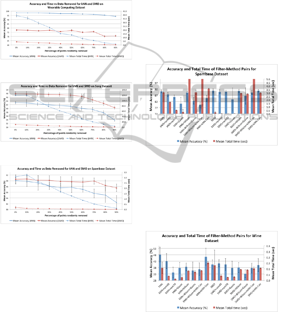
remaining data to each classifier. A typical result
obtained with the Wearable Computing dataset is
shown in Figure 1, for the classification accuracy
(left vertical axis) and the total running time (right
vertical axis). Total time refers to the sum of the
times taken for training data condensation, training
time, and testing time (results for the three
individual timings will be presented in a following
section). In this and all other experiments the
classification accuracies and timings were obtained
by the method of K-fold cross-validation (or
method) with a value of K = 10 (Toussaint, 1974).
This means that for each of the classifiers and
condensing methods tested the procedure for
estimating the classification accuracy for each fold
was the following. Let {X} denote the entire dataset.
The ith fold is obtained by taking the ith 10% of {X}
as the testing set, denoted by {X
TS-i
}, and the
remaining 90% of the data as the training set,
denoted by {X
TR-i
}. Estimates of the
misclassification accuracy of any classifier are then
obtained by training the classifier on {X
TR-i
}, and
testing it on {X
TS-i
}, for i = 1, 2, …, 10, yielding a
total of ten estimates. Similarly, when estimating the
classification accuracy of an editing (or condensing)
method, the editing (or condensing) is first applied
to {X
TR-i
}, and the resulting edited (condensed) set is
used to classify {X
TS-i
}. Finally, in all cases the
average of the ten estimates obtained in this way is
calculated. Thus the results shown in the figures are
the mean values over the ten folds. This method also
permits the computation of standard deviations (over
the ten folds) to serve as indicators of statistically
significant differences between the means. The error
bars in the figures indicate ± one standard deviation.
All seven datasets exhibit similar behaviour to that
depicted in Figure 1, with respect to how the
classification accuracy varies as a function on the %
of training data removed. The classification accuracy
results are not unanimous, but favour k-NN over
SMO, the latter having significantly better accuracy
than k-NN only for the Song data (Figure 2). For the
Letter Image, Wearable Computing, and MAGIC
Gamma datasets k-NN did significantly better
(example: Figure 1). Furthermore, for some of the
SpeedingupSupportVectorMachines-ProbabilisticversusNearestNeighbourMethodsforCondensingTrainingData
367
datasets such as the Spam, Wine, and Handwritten
Digits data there are no significant differences
between SMO and k-NN. For the Spambase data
SMO is significantly better only when more than
60% of the data are discarded (see Figure 3).
Figure 1: Accuracy and time vs % training data removed
by random sampling for Wearable Computing data.
Figure 2: Accuracy and time versus % of training data
removed by blind random sampling for Song data.
Figure 3: Accuracy and time versus % of training data
removed by blind random sampling for Spambase data.
With respect to the total time taken by SMO and k-
NN, in all the datasets, SMO takes considerably less
running time than k-NN, and all show behaviour
similar to the curves in Figures 1-3. For example, if
70% of the data are discarded then k-NN runs about
five times faster (and SMO about ten times faster)
than when all the data is used for training. This is
not too surprising since k-NN runs in O(N
2
)
expected time and SMO is able to run faster in
practice depending on the structure of the data.
4.3 The Condensing Classifiers
Experiments were done applying various training
data condensation classifiers to reduce the size of
the training data that was fed to both the SMO and k-
NN classifiers. The condensing classifiers tried
were: (1) Gaussian condensation, (2) Wilson editing,
(3) Wilson editing+Gaussian condensation, (4)
Wilson editing+k-NN condensation, and (5) k-NN
condensation. Figures 4-10 show the per-cent mean
accuracy and mean total running times (in seconds)
for all the five condensation classifiers, plus the
results for blind random sampling obtained by
discarding 40% (rem40) and 70% (rem70) of the
training data. In all the figures ‘Con’ indicates
condensation, ‘Wilson’ denotes Wilson smoothing,
and ‘Gauss’ stands for Gaussian condensation.
Figure 4: Accuracy and total time of condensing algorithm
methods for the Spambase data.
Perusal of the figures reveals that none of the
condensing methods improves the accuracy of the
classifiers that do not use condensing. With some of
the datasets the accuracy remains unchanged, such
as for the Wearable Computing data in Figure 7, and
the Handwritten Digits in Figure 8. For other
datasets accuracy suffers considerably, as with the
Wine data in Figure 5, and the Song data in Figure 9.
Figure 5: Accuracy and total time of condensing algorithm
methods for the Wine data.
With k-NN classification, random removal of 70%
ICPRAM2014-InternationalConferenceonPatternRecognitionApplicationsandMethods
368
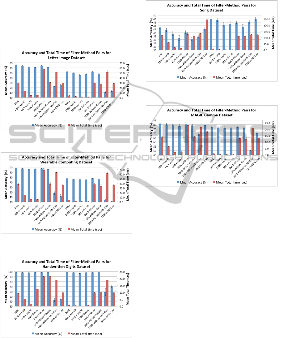
of the training set, and Gaussian condensation were
the fastest methods for all the datasets other than the
Handwritten Digits. Similar relative behavior was
observed with SMO. However, in all cases the
running times for condensing with SMO were much
smaller than those for condensing with k-NN.
Figure 6: Accuracy and total time of condensing algorithm
methods for the Letter Image data.
Figure 7: Accuracy and total time of condensing algorithm
methods for the Wearable Computing data.
Figure 8: Accuracy and total time of condensing algorithm
methods for the Handwritten Digits data.
In Figures 4-10 the times plotted are total times:
condensing time + training time + testing time. One
of the main goals of this research is to compare the
testing times of the various classifiers, since these
Figure 9: Accuracy and total time of condensing algorithm
methods for the Song data.
Figure 10: Accuracy and total time of condensing
algorithm methods for the MAGIC Gamma data.
reflect the speed of the classifier on all future data.
However, if the condensing times and training times
dominate the testing time, then the total times listed
in the figures may hide the testing times. Therefore a
breakdown of the individual times was also plotted
for all the experiments. Space does not permit
including all the figures, and therefore an example is
offered for the Magic Gamma data in Figure 11.
Note from Figure 10 that the classifiers with the
smallest total times are: SMO, SMO+rem40,
SMO+rem70, and SMO+Gauss. Furthermore their
accuracies are not significantly different. Therefore
the classifiers with the fastest testing times would be
preferred in this case.
Figure 11 shows the breakdown of condensing,
training, testing, and total time for the MAGIC
Gamma data on a linear scale in seconds. This figure
clearly shows how large the testing time for k-NN is
compared to all other classifiers, thus making it
difficult to compare the four classifiers of main
interest. To zoom in on their performance the data
from Figure 11 are shown on a logarithmic scale in
Figure 12, where it can be clearly seen that SMO
runs faster when pre-processed by rem40 or rem60,
but not when pre-processed by Gaussian
SpeedingupSupportVectorMachines-ProbabilisticversusNearestNeighbourMethodsforCondensingTrainingData
369
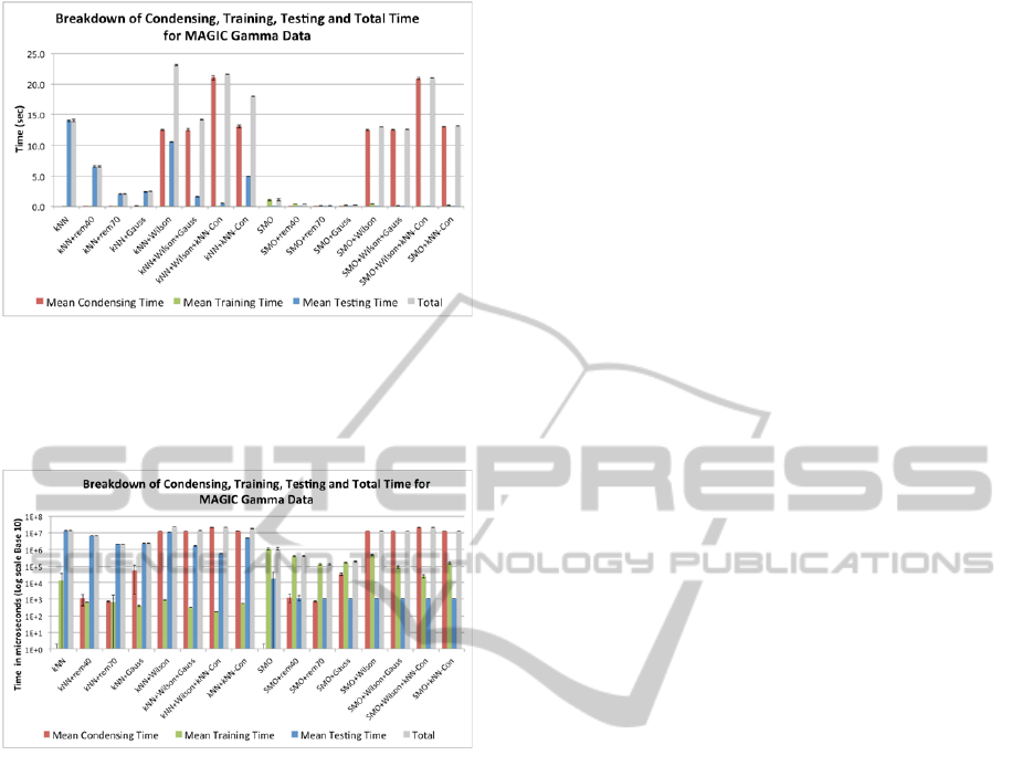
Figure 11: Breakdown of condensing, training, testing, and
total time for the MAGIC Gamma data.
condensation. Similar behaviour is observed with the
other six datasets.
Figure 12: The data of Figure 11 on a logarithmic scale.
5 CONCLUSIONS
One of the main conclusions that can be made from
the experiments reported here is that blind random
sampling is surprisingly good and robust. For all the
datasets, as much as 70% to 80% of the data may be
discarded, without incurring any significant decrease
in the classification accuracy. Furthermore, for six of
the seven datasets, discarding 70% of the data at
random in this way made k-NN run about five times
faster, and SMO about ten times faster. Since this
method is so simple and requires so little
computation time we believe that it should play a
role as a pre-processing step for speeding up SVMs.
Previous research has shown that SVMs perform
better than k-NN. However, some of the
comparisons have used synthetically generated data
that does not resemble real world data. On the other
hand, the results of the present study with seven
real-world datasets tell a different story. SMO is
significantly better only for the Song data, whereas
k-NN does better for the Letter Images, Wearable
Computing, and Magic Gamma datasets. For the
other three datasets (Spam, Wine, and Handwritten
Digits) there are no significant differences between
SMO and k-NN. In future research we hope to
discover structural features of the data that predict
when SMO is expected to outperform k-NN.
One of the goals of this research was too test
how much Wilson editing improves the accuracy of
classifiers in practice. It was found that for all seven
datasets that using Wilson editing as a pre-
processing step to either SVM or k-NN, yielded no
statistically significant improvement in accuracy.
Furthermore, except for the Wine and Song datasets
Wilson editing incurs a considerable additional cost
in the editing (condensing) time, although it can
speed up the training and testing times.
Another main goal of this research project was to
compare the new proposed method for condensing
training data in O(N) worst-case time: Gaussian
condensation. This probabilistic method falls in the
category of guided (or intelligent) random sampling
and is almost as fast as blind random sampling. The
results of this study show that Gaussian
condensation is competitive with 70% blind random
sampling, with respect to both accuracy and running
time, relative to the other methods tested. However,
the main overall conclusion of this study is that blind
random sampling is the best overall method for
speeding up support vector machines.
ACKNOWLEDGEMENTS
This research was supported by a grant from the
Provost's Office of New York University Abu Dhabi
in the United Arab Emirates. The authors are
grateful to the University of California at Irvine for
making available their large collection of data at the
Machine Learning Repository.
REFERENCES
Bache, K., Lichman, M., 2013. UCI Machine Learning
Repository [http://archive.ics.uci.edu/ml]
Bakir, G. H, Bottou, L., Weston, J., 2004. Breaking SVM
complexity with cross-training. In Advances in Neural
Information Processing Systems 17 (NIPS-2004), Dec.
13-18, 2004, Vancouver, Canada], pp. 81-88.
Bordes, A., Ertekin, S., Weston, J., Bottou, L., 2005. Fast
kernel classifiers with online and active learning. J. of
Machine Learning Research, vol. 6, pp. 1579-1619.
Almeida, M. B., Braga, A. P., Braga, J. P., 2000. SVM-
KM: speeding SVMs learning with a priori cluster
ICPRAM2014-InternationalConferenceonPatternRecognitionApplicationsandMethods
370

selection and k-means. In: Proc. of the 6th Brazilian
Symposium on Neural Networks, pp. 162–167.
Chen, J., Zhang, C., Xue, X., Liu, C.-H., 2013. Fast
instance selection for speeding up support vector
machines. Knowledge-Based Systems, vol. 45, pp. 1-7.
Chen, J., Liu, C.-L., 2011. Fast multi-class sample
reduction for speeding up support vector machines.
Proceedings of the IEEE International Workshop on
Machine Learning for Signal Processing, Beijing,
China, September 18-21.
Chen, J., Chen, C., 2002. Speeding up SVM decisions
based on mirror points. Proc. 6
th
International Conf.
Pattern Recognition, vol. 2, pp. 869-872.
Devroye, L., 1981. On the inequality of Cover and Hart in
nearest neighbour discrimination. IEEE Trans. Pattern
Analysis and Machine Intelligence, vol. 3, pp. 75–78.
Hart, P. E., 1968. The condensed nearest neighbour rule.
IEEE Trans. Infor. Theory, vol. 14, pp. 515–516.
Kawulok, M., Nalepa, J., 2012. Support vector machines
training data selection using a genetic algorithm. In
G.L. Gimel’farb et al. (Eds.): Structural, Syntactic,
and Statistical Pattern Recognition, LNCS 7626, pp.
557–565.
Keerthi, S. S., Shevade, S. K., Bhattacharyya, C., Murthy,
K. R. K., 2001. Improvements to Platt’s SMO
algorithm for SVM classifier design. Neural
Computation, vol. 13, pp. 637-649.
Lee, Y. L., Mangasarian, O. L., 2001. RSVM: Reduced
support vector machines. In Proceedings of the First
SIAM International Conference on Data Mining,
SIAM, Chicago, April 5-7, (CD-ROM).
Li, X., Cervantes, J., Yu, W., 2012. Fast classification for
large datasets via random selection clustering and
Support Vector Machines. Intelligent Data Analysis,
vol. 16, pp. 897-914.
Liu, X., Beltran, J. F., Mohanchandra, N., Toussaint, G.
T., 2013. On speeding up support vector machines:
Proximity graphs versus random sampling for pre-
selection condensation. Proc. International Conf.
Computer Science and Mathematics, Dubai, United
Arab Emirates, Jan. 30-31, Vol. 73, pp. 1037-1044.
Ng W. Q., Dash, M., 2006. An evaluation of progressive
sampling for imbalanced datasets. In Sixth IEEE
International Conference on Data Mining Workshops,
Hong Kong, China. 2006.
Panda, N., Chang, E. Y., Wu, G., 2006. Concept boundary
detection for speeding up SVMs. Proc. 23
International Conf. on Machine Learning, Pittsburgh.
Platt, J. C., 1998. Fast training of support vector machines
using sequential minimial optimization. In Advances
in Kernel Methods: Support Vector Machines, B.
Scholkopf, C. Burges, and A. Smola, Eds., MIT Press.
Portet, F., Gao, F., Hunter, J., Quiniou, R., 2007.
Reduction of large training set by guided progressive
sampling: Application to neonatal intensive care data.
Proc. of Intelligent Data Analysis in Biomedicine and
Pharmacology, Amsterdam, pp. 43-44 .
Provost, F., Jensen, D., Oates, T., 1999. Efficient
progressive sampling. In Fifth ACM SIGKDD
International Conference on Knowledge Discovery
and Data Mining, San Diego, USA, 1999.
Sriperumbudur, B. K., Lanckriet, G., 2007. Nearest
neighbour prototyping for sparse and scalable support
vector machines. Technical Report No. CAL-2007-02,
University of California San Diego.
Toussaint, G. T., Berzan, C., 2012. Proximity-graph
instance-based learning, support vector machines, and
high dimensionality: An empirical comparison.
Proceedings of the Eighth International Conference
on Machine Learning and Data Mining, July 16-19,
2012, Berlin, Germany. P. Perner (Ed.): LNAI 7376,
pp. 222–236, Springer-Verlag Berlin Heidelberg.
Toussaint, G. T., 2005. Geometric proximity graphs for
improving nearest neighbour methods in instance-
based learning and data mining. International J.
Computational Geometry and Applications, vol. 15,
April, pp. 101-150.
Toussaint, G. T., 1974. Bibliography on estimation of
misclassification. IEEE Transactions on Information
Theory, vol. 20, pp. 472-479.
Vapnik, V., 1995. The Nature of Statistical Learning
Theory, Springer-Verlag, New York, NY.
Wang, Y., Zhou, C. G., Huang, Y. X., Liang, Y. C., Yang,
X. W., 2006. A boundary method to speed up training
support vector machines. In: G. R. Liu et al. (eds),
Computational Methods, Springer, Printed in the
Netherlands, pp. 1209–1213.
Wilson, D. L., 1973. Asymptotic properties of nearest
neighbour rules using edited-data. IEEE Trans.
Systems, Man, and Cybernetics, vol. 2, pp. 408–421.
Witten, I., Frank, E., 2000. WEKA: Machine Learning
Algorithms in Java. In Data Mining: Practical
Machine Learning Tools and Techniques with Java
Implementations, Morgan Kaufmann, pp. 265-320.
SpeedingupSupportVectorMachines-ProbabilisticversusNearestNeighbourMethodsforCondensingTrainingData
371
