
A Hierarchical Clustering based Heuristic for Automatic Clustering
Franc¸ois LaPlante
1
, Nabil Belacel
2
and Mustapha Kardouchi
1
1
Department of Computer Sciences, Universit´e de Moncton, E1A 3E9, Moncton, NB, Canada
2
National Research Council - Information and Communications Technologies, E1A 7R9, Moncton, NB, Canada
Keywords:
Data-mining, Automatic Clustering, Unsupervised Learning.
Abstract:
Determining an optimal number of clusters and producing reliable results are two challenging and critical
tasks in cluster analysis. We propose a clustering method which produces valid results while automatically
determining an optimal number of clusters. Our method achieves these results without user input pertaining
directly to a number of clusters. The method consists of two main components: splitting and merging. In
the splitting phase, a divisive hierarchical clustering method (based on the DIANA algorithm) is executed and
interrupted by a heuristic function once the partial result is considered to be “adequate”. This partial result,
which is likely to have too many clusters, is then fed into the merging method which merges clusters until
the final optimal result is reached. Our method’s effectiveness in clustering various data sets is demonstrated,
including its ability to produce valid results on data sets presenting nested or interlocking shapes. The method
is compared with cluster validity analysis to other methods to which a known optimal number of clusters is
provided and to other automatic clustering methods. Depending on the particularities of the data set used, our
method has produced results which are roughly equivalent or better than those of the compared methods.
1 INTRODUCTION
Data clustering, also known as cluster analysis, seg-
mentation analysis, taxonomy analysis (Gan, 2011),
is a form of unsupervised classification of data points
into groups called clusters. Data points in a same clus-
ter should be a similar to each other as possible and
data points in different clusters should be as dissimilar
as possible (Jain et al., 1999).
One common problem across many clustering
methods is determining the correct (optimal) number
of clusters. One prevalent method to determine an op-
timal number of clusters involves the use of validity
indices. Cluster validity indices are a value computed
based on a clustering result and represent a relative
quality of this clustering. Often, a clustering method
will be applied to the target data set a number of times
with a different number of clusters and a validity in-
dex will be computed for each resulting clustering.
The result which leads to the best index value will be
taken as being the most optimal. Given n the number
of data points, the number of clusters to try can be a
sequence (often from 2 to
√
n), all possible values (1
to n), or a selection of specific values or ranges based
on prior knowledge of the data set.
Even with the use of cluster validity indices, it is
still required to cluster the data many times and com-
pare the results to determine the optimal clustering.
There is a group of clustering algorithms, called auto-
matic clustering algorithms, which determine an opti-
mal number of clusters automatically. These methods,
although generally more complex and time consum-
ing, do not need to be run more than once. Some of
these algorithms, such as Y-means(Guan et al., 2003),
still require an initial number of clusters from which
to start. Others, such as the method proposed by Mok
et. al. (Mok et al., 2012), hereafter referred to as
RAC, requires no user input at all regarding the num-
ber of clusters. Our goal is to develop an automatic
clustering algorithm which requires minimal user in-
put and more specifically does not require to be pro-
vided a target number of clusters or an initial number
of clusters from which to start.
2 RELATED WORKS
2.1 Types of Clustering
Clustering methods can be categorized in many ways
such as hard or fuzzy, hierarchical or partitional, and
as combinations of these types.
201
LaPlante F., Belacel N. and Kardouchi M..
A Hierarchical Clustering Based Heuristic for Automatic Clustering.
DOI: 10.5220/0004925902010210
In Proceedings of the 6th International Conference on Agents and Artificial Intelligence (ICAART-2014), pages 201-210
ISBN: 978-989-758-015-4
Copyright
c
2014 SCITEPRESS (Science and Technology Publications, Lda.)

2.1.1 Hard vs. Fuzzy Clustering
Hard clustering, also called crisp clustering, is a type
of clustering where every datum belongs to one and
only one cluster. In contrast, fuzzy clustering is a
form of clustering where data belong to multiple clus-
ters according to a membership function (Gan, 2011).
Hard clustering is generally simpler to implement and
has lower time complexity. Hard clustering performs
well with linearly separable data but often does not
perform very well with non linearly separable data,
outliers, or noise. Fuzzy clustering often has a larger
memory footprint as it often requires a c×n matrix to
store memberships, where c is the number of clusters
and n is the number of data points. Fuzzy clustering
is able to handle non-linearly separable data as well
as outliers, and noise better than hard clustering.
2.1.2 Hierarchical vs. Partitional Clustering
A hierarchical clustering method yields a dendrogram
representing the nested grouping of patterns and sim-
ilarity levels at which groupings change (Jain et al.,
1999). A partitional clustering method yields a single
partition of the data instead of a clustering structure,
such as the dendrogram produced by a hierarchical
method (Gan, 2011).
2.1.3 Automatic Clustering
Automatic clustering is a form of clustering where
the number of clusters c is unknown and determining
its optimal value is left up to the clustering method.
Some automatic clustering methods may require an
initial number of clusters, from which clusters will
be split and merged until a pseudo-optimal number of
clusters is achieved. Other methods require no initial
value or additional information regarding the num-
ber of clusters and will determine a pseudo-optimal
value without any user input. Other parameters, such
as a fuzzy constant (for fuzzy clustering algorithms)
or thresholds, may still be required, but are generally
kept to minimum or are optional with good default
values.
2.2 Validation Methods
As clustering is by definition an unsupervised
method, there is generally no training data with
known output values with which to compare results.
As such, it requires a different approach to evaluat-
ing its results. The quality of clustering is evaluated
using a validity index, which is a relative measure of
clustering quality based on a number of parameters.
There are many clustering validity indices, but the ap-
proach to using them generally remains the same and
is as follows:
1. Use fixed values for all parameters other than c
the number of clusters.
2. Iteratively cluster the data set with the clustering
method being evaluated with varying values of c
(often from 2 to
√
2).
3. Calculate the validity index for every clustering
generated by 2.
4. The clustering for which the validity index
presents the best value is considered to be “op-
timal”.
A good index must consider compactness (high intra-
cluster density), separation (high inter-cluster dis-
tance or dissimilarity) and the geometric structure of
data (Wu and Yang, 2005).
2.2.1 Xie and Beni Index
Xie and Beni have proposed a validity index which
relies on two properties, compactness and separation
(Xie and Beni, 1991), which was later modified by
Pal and Bezdek (Pal and Bezdek, 1995). This index is
defined by
V
XB
=
∑
c
i=1
∑
n
k=1
u
m
ik
kx
k
−v
i
k
2
n(min
i, j∈c,i6= j
{v
i
−v
j
})
(1)
where u is a n×c matrix such that u
ik
is the mem-
bership of object k to cluster i, m is a fuzzy constant,
x
k
are data points and v
i
are clusters (represented by
their centroids).
The numerator of the equation, which is equiva-
lent to the least squared error, is an indicator of com-
pactness of the fuzzy partition, while the denominator
is an indicator of the strength of the separation be-
tween the clusters. A more optimal partition should
produce a smaller value for the compactness and well
separated clusters should produce a higher value for
the separation. An optimal number of clusters c is
generally found by solving min
2≤c≤n−1
V
XB
(c).
2.2.2 Fukuyama and Sugeno Index
Fukuyama and Sugeno also proposed a validity index
based on compactness and separation (Fukuyama and
Sugeno, 1989) defined by:
V
FS
= J
m
−K
m
=
c
∑
i=1
n
∑
k=1
u
m
ik
kx
k
−v
i
k
2
−
c
∑
i=1
n
∑
k=1
u
m
ik
kv
i
− ¯vk
2
(2)
where J
m
represents a measure of compactness, K
m
represents a measure of separation between clusters
ICAART2014-InternationalConferenceonAgentsandArtificialIntelligence
202

and ¯v is the mean of all cluster centroids. An opti-
mal number of clusters c is generally found by solving
min
2≤c≤n−1
V
FS
(c).
2.2.3 Kwon Index
Kwon extends the index of Xie and Beni’s validity
function to eliminate its tendency to monotonically
decrease when the number of clusters approaches the
number of data points. To achieve this, a penalty
function was introduced to the numerator of Xie and
Beni’s original validity index. The resulting index
was defined as
V
K
=
∑
n
j=1
∑
c
i=1
u
m
ij
kx
j
−v
i
k
2
+
1
c
∑
c
i=1
kv
i
− ¯vk
2
min
i,k∈c,i6=k
kv
i
−v
k
k
2
(3)
An optimal number of clusters c is generally found
by solving min
2≤c≤n−1
V
K
(c).
2.2.4 PBM Index
Pakhira and Bandyopadhyay (Pakhira et al., 2004)
proposed the PBM index, which was developed for
both hard and fuzzy clustering. The hard clustering
version of the PBM index is defined by
V
PBM
=
1
c
·
E
1
E
c
·D
c
2
(4)
where
E
c
=
c
∑
k=1
E
k
(5)
and
E
k
=
n
∑
j=1
kx
j
−v
k
k (6)
with v
k
being the centroid of the data set and
D
c
= max
i, j∈c
kv
i
−v
j
k (7)
An optimal number of clusters c is generally found
by solving max
2<c<n−1
V
PBM
(c).
2.2.5 Compose within and between Scattering
The CWB index proposed by Rezaee(Rezaee et al.,
1998) focusing on both the density of clusters and
their separation. Although meant to evaluate fuzzy
clustering results, it can be used to evaluate hard clus-
tering by generating a partition matrix u such that
memberships have values of 1 or 0 (is a member or
is not a member).
Given a fuzzy c-partition of the data set X =
{x
1
,x
2
,...,x
n
|x
i
∈ R
p
} with c cluster centers v
i
, the
variance of the pattern set X is called σ(X) ∈ R
p
with
the value of the pth dimension defined as
σ
p
x
=
1
n
n
∑
k=1
(x
p
k
− ¯x
p
)
2
(8)
where ¯x
p
is the pth element of the mean of
¯
X =
∑
n
k=1
x
k
/n.
The fuzzy variation of cluster i is called σ(v
i
) ∈R
p
with the pth value defined as
σ
p
v
i
=
1
n
n
∑
k=1
u
ik
(x
p
k
−v
p
i
)
n
(9)
The average scattering for c clusters is defined as
Scat(c) =
1
n
∑
c
i=1
kσ(v
i
)k
kσ(X)k
(10)
where kxk = (x
T
·x)
1/2
A dissimilarity function Dis(c) is defined as
Dis(c) =
D
max
D
min
c
∑
k=1
c
∑
z=1
kv
k
−v
z
k
!
−1
(11)
where D
max
= max
i, j∈{2,3,...,c}
{kv
i
−v
j
k} is the
maximum dissimilarity between the cluster proto-
types. The D
min
has the same definition as D
max
, but
for the minimum dissimilarity between the cluster
prototypes.
The compose within and between scattering index
is now defined by combining the last two equations:
V
CWB
= αScat(c) + Dis(c) (12)
Where α is a weighting factor.
An optimal number of clusters c is generally found
by solving min
2<c<n−1
V
CWB
(c).
2.2.6 Silhouettes Index
Rousseeuw introduced the concept of silhouettes
(Rousseeuw, 1987) which represent how well data lie
within their clusters. The silhouette value of a datum
is defined by
S(i) =
1−a(i)/b(i), a(i) < b(i)
0, a(i) = b(i)
b(i)/a(i) −1, a(i) > b(i)
(13)
which can also be written as
S(i) =
b(i) −a(i)
max{a(i),b(i)}
(14)
AHierarchicalClusteringBasedHeuristicforAutomaticClustering
203

where a(i) is the average dissimilarity between a point
i and all other points in its cluster and b(i) is the av-
erage dissimilarity between a point i and all points
of the nearest cluster to which point i is no assigned.
The silhouette index for a given cluster is the aver-
age silhouette for all points within that cluster and the
silhouette index of a clustering is the average of all
silhouettes in the data set:
V
S
=
n
∑
i=1
S(i)/n. (15)
An optimal number of clusters c is generally found
by solving max
2≤c≤n−1
V
S
(c).
3 PROPOSED METHOD
The proposed method, Heuristic Divisive Analysis
(HDA), consists of two phases: splitting and merg-
ing. The first phase splits the data set into a num-
ber of clusters, often leading to more cluster than
optimal. The second phase merges (or links) clus-
ters, leading to a more optimal clustering. The rea-
son for this two-step approach is to address one of
the larger drawbacks of hard clustering; poor perfor-
mance when dealing with data which is not linearly
separable. Both steps use different approaches to
computing the dissimilarity between clusters, which
allows for the creation of non-elliptical clusters which
may be nested or interlocked.
3.1 Splitting
The splitting algorithm is a divisive hierarchical
method based on the DIANA clustering algorithm
(Kaufman and Rousseeuw, 1990). However, the pro-
posed method employs a heuristic function to inter-
rupt the hierarchical division of the data set once an
“adequate” clustering for this step has been reached.
3.1.1 DIANA
DIANA (DIvisive ANAlysis) is a divisive hierar-
chical clustering algorithm based on the idea of
MacNaughton-Smith et al. (MacNaughton-Smith,
1964). Given X = x
1
,x
2
,...,x
n
a data set consisting of
n records and beginning with all points being in one
cluster, the algorithm will alternate between separat-
ing the cluster in two and selecting the next cluster to
split until every point has become its own cluster. To
split a cluster in two, the algorithm must first find the
point with the greatest average dissimilarity to the rest
of the records. The average dissimilarity of a record
x
i
with regards to X is defined as
D
i
=
1
n−1
n
∑
j=1, j6=i
D(x
i
,xj) (16)
where D(x,y) is a dissimilarity metric (in this
case, we use Euclidean distance). Given D
max
=
max
0≤i≤n−1
D
i
, x
max
is the point with the greatest av-
erage dissimilarity which is then split from the clus-
ter. We then have two clusters: C
1
= {x
max
} and
C
2
= X\C
1
. Next, the algorithm checks every point
in C
2
to determine whether or not it should be moved
to C
1
. To accomplish this, the algorithm must com-
pute the dissimilarity between x and C
1
as well as the
dissimilarity between x and C
2
\x. The dissimilarity
between x and C
1
is defined as
D
C
1
(x) =
1
|C
1
|
∑
y∈C
1
D(x,y),x ∈C
2
(17)
where |C
1
| denotes the number of records in C
1
. The
dissimilarity between x and C
2
\x is defined as
D
C
2
(x) =
1
|C
2
−1|
∑
y∈C
2
,y6=x
D(x,y),x ∈C
2
(18)
If D
C
1
< D
C
2
, then x is moved from C
2
to C
1
. This
process is repeated until there are no more records in
C
2
which should be moved to C
1
.
To select the next cluster to separate, the algorithm
will chose the cluster with the greatest diameter. The
diameter of a cluster is defined as
Diam(C) = max
x,y∈C
D(x,y) (19)
3.1.2 Heuristic Stopping Function
The first phase in our method consists of running
the DIANA algorithm with a heuristic function in or-
der to stop it once an “adequate” clustering has been
reached. This function consists of first calculating
the average intra-cluster dissimilarity (again, we use
Euclidean distance) of each cluster, defined as
AvgIntraClusterDistance(C) =
∑
x∈C
D(x, ¯x)
|C|
(20)
where ¯x denotes the mean of all points in cluster C.
The heuristic index for this clustering is the average
of all the average intra-cluster dissimilarities. If the
heuristic index for this clustering is lower than that
of the previous clustering, the current clustering is
considered the most optimal to date. Otherwise, we
have reached our “adequate” clustering at the previ-
ous step, but we will continue running the DIANA
algorithm for a set number of iterations as a preventa-
tive measure against falling into a local optimum. We
ICAART2014-InternationalConferenceonAgentsandArtificialIntelligence
204

chose this rather simple heuristic instead of one of the
many known validity indices because it allowed us to
decrease the complexity (as it uses values which our
implementation had already calculated) and still pro-
duced good results.
3.2 Merging
The splitting phase’s result can be non-optimal. This
is especially likely when data sets contain clusters
which are not linearly separable or have irregular
shapes. In these cases, the “adequate” clustering will
usually contain instances where what should be one
single cluster is divided into many. These many clus-
ters will be very close to each other in relation to the
other clusters and it is the goal of this merging phase
to collect them into optimal clusters.
For each pair of clusters, we calculate the average
nearest neighbor dissimilarity, defined as
AvgNearestNeighbor(C) =
∑
x∈C
min
y∈C,y6=x
D(x,y)
|C|
(21)
for both clusters and keep the greater of both values
as our merging dissimilarity threshold M
T
. We then
go through each pair of objects with one object from
each cluster and if we find a pair where the dissimi-
larity between the two objects is less than the merg-
ing dissimilarity threshold (multiplied by a constant),
then the two clusters are merged. We express the test
for merging as
CanMerge(C
1
,C
2
) =
(
true, ∃x ∈C
1
,∃y ∈C
2
|D(x,y) < M
T
·K
false, otherwise
(22)
Where K is a merging constant.
Once all merges are completed, we are left with
the final clustering. The value of the merging con-
stant can be adjusted depending on the data set and
we have found experimentally that a value of 2 gener-
ally produces good results.
We havealso tested an alternativemerging method
based on the Y-means approach to merging. Because
the Y-means algorithm uses dissimilarities between
cluster centroids, merging clusters will relocate the
centroids in such a way that is detrimental to our
method. To avoid this drawback, we link clusters by
attributing them labels instead of merging them until
all pairs are linked, after which we merge all linked
clusters. We express the test for linking as
CanLink(C
1
,C
2
) =
(
true D(C
1
,C
2
) ≤ (σ
C
1
·σ
C
2
) ·L
false otherwise
(23)
where σ
C
i
is the standard deviation of the dissimilarity
between the objects in a cluster C
i
to the centroid of
that cluster and L is a linking constant. The value
of the linking constant can be adjusted depending on
the data set and we have found that a value of 0.5
generally produces good results with our method.
4 RESULTS
The proposed method was tested with five data sets.
The results were compared to the Y-means, fuzzy c-
means (Bezdek et al., 1984) and RAC algorithms us-
ing the Xie & Beni, Fukuyama & Sugeno, Kwon,
CWB, PBM and Silhouette validation indices.
4.1 Data Sets
The first data set was the Iris data set (Fisher, 1936),
composed of 150 elements in four dimensions belong-
ing to three categories of 50 elements each; however,
two of the three categories of the data set are so close
as to generally be clustered together.
The second data set, or “nested circles” data set, is
composed of 600 elements in two dimensions belong-
ing to two groups. The first group, of 100 elements,
is a full circular shape in the center of the plane. The
second group, of 500 elements, is a circular shell sur-
rounding the first group. As the centroids of both
clusters are approximately identical, it is difficult for
clustering methods which use cluster centroids (such
as Y-means and fuzzy c-means) to produce an appro-
priate clustering.
The third data set, or “nested crescents” data set,
is composed of 500 elements in two dimensions be-
longing to two groups of 250 elements each. The two
groups form opposing semi-circles which are offset
and inset in such a way that one tip of each semi-circle
is nested within the other semi-circle.
The fourth data set, or “five groups” data set, is
composed of 1500 elements in two dimensions be-
longing to five groups of 300 elements each. Each
group is a roughly circular with an approximately
Gaussian distribution. The groups are spread in such
a way as to have two pairs of tightly adjacent clusters.
The fifth data set or “Aggregation” data set is a
testing data set proposed by Gionis et.al. (Gionis
et al., 2007). This data set presents 7 roughly ellip-
tical groupings, one of which has a concave indenta-
tion. Two pairs of these groups a linked by narrow
lines of data points.
AHierarchicalClusteringBasedHeuristicforAutomaticClustering
205
4.2 Clustering Results
We have compared our method to the Y-means al-
gorithm, another hard automatic clustering method
based on the well-known k-means algorithm. Y-
means requires an initial number of clusters, as such
we provided it with the known optimal number of
clusters or the best approximations thereof.
We have also compared our method to the fuzzy
c-means algorithm. Although this method belongs
to the category of fuzzy clustering, we compared our
method to it as our method should be able to correctly
treat non-linearly separable data and comparison with
a fuzzy method could prove interesting.
As well as the previous two methods, we have
compared our method to the RAC method. This
method makes use of the fuzzy c-means algorithm as
well as graph partitioning concepts to arrive at a hard
partition. This automatic clustering method should
also be able to correctly treat non-linearly separable
data but has a greater time complexity.
Of the validity indices used, Xie & Beni,
Fukuyama & Sugeno, Kwon, and CWB should be
minimized (lower values indicates a better cluster-
ing) while PBM and Silhouette should be maximized
(higher value indicates a better clustering).
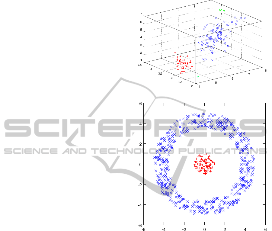
4.2.1 Iris Data Set
Fig. 1 shows the result of clustering the Iris data
set with our method. We can discern four clusters,
two of which contain one and two members respec-
tively. These two clusters are considered as outliers
and the remaining two clusters then approximately
correspond to the expected results.
Table 1 shows the validation results of our method
and the compared methods for the Iris data set. The
results for the proposed method (HDA) were calcu-
lated after removing all outliers. We notice that for
the XB, Kwon, CWB, and PBM indices, although our
method does not produce the best validation result, its
results are very near the best. For the XB and Kwon
indices, our method outperformed the other hard clus-
tering methods. The small variations in results be-
tween our method and the others are partly due to the
data points eliminated when removing outliers.
4.2.2 Nested Circles Data Set
Fig. 2 shows the result of clustering the nested circles
data set with our method and Table 2 shows the vali-
dation results of our method and the compared meth-
ods for the nested circles data set.
We can observe that the two clusters are correctly
identified. However, the validation indices for our
Figure 1: Clustering result on Iris data set.
Figure 2: Clustering result on nested circles data set.
method and RAC (which produced the same cluster-
ing) are all much worse than those of Y-means and
fuzzy c-means which did not correctly identify the
clusters (see Fig. 3). This is in part due to the fact
that most of these indices use the centroids of clus-
ters to compute dissimilarities, which is also at least
in part the reason why Y-means and fuzzy c-means
did not produce good results.
4.2.3 Nested Crescents Data Set
Fig. 4 shows the result of clustering the nested cres-
cents data set with our method. We can see that the
two clusters are correctly identified.
Table 3 shows the validation results of our method
and the compared methods for the nested crescents
data set. The RAC method has no values for this data
set as it clustered the entire data set into a single clus-
ter.
ICAART2014-InternationalConferenceonAgentsandArtificialIntelligence
206
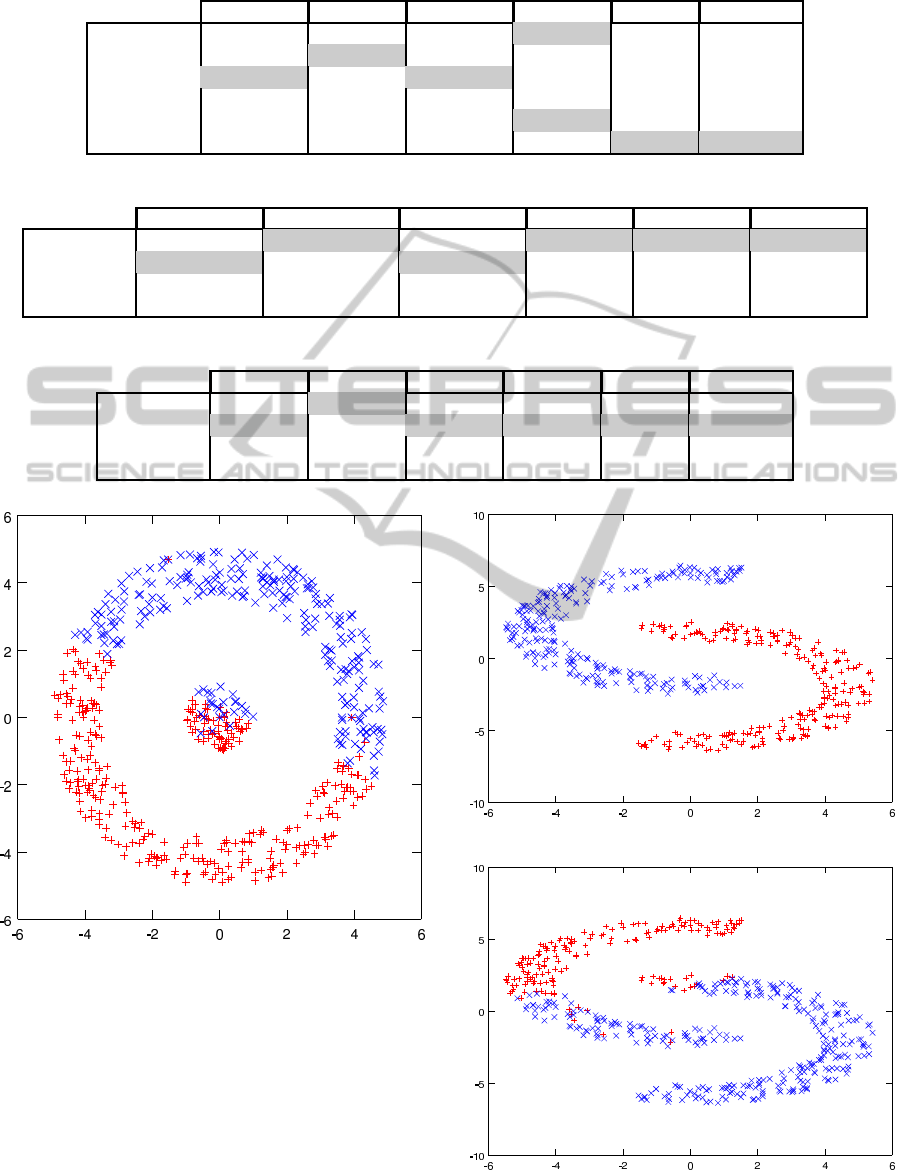
Table 1: Iris data set validation results.
XB FS Kwon CWB PBM Silhouette
KMP (c=2) 0.0654087 −592.227 10.0613 0.503325 23.8917 0.690417
KMP (c=3) 1.55946 −789.946 239.56 2.7801 14.4217 0.561084
FCM (c=2) 0.0544162 −530.501 8.41243 0.503334 17.1528 0.685031
FCM (c=3) 0.137036 −509.939 21.966 1.34779 14.8009 0.558518
RAC 0.0654087 −592.227 10.0613 0.503325 23.8917 0.690417
HDA 0.061941 −568.303 9.35532 0.508643 24.2696 0.697063
Table 2: Nested circles data set validation results.
XB FS Kwon CWB PBM Silhouette
KMP (c=2) 0.45743 −3367.37 274.708 0.422658 8.53994 0.340658
FCM (c=2) 0.318881 −2173.72 191.578 0.427173 6.34011 0.338348
RAC 2600.64 −0.908002 1.56039e6 25.7067 0.00151379 −0.0477678
HDA 2600.64 −0.908002 1.56039e6 25.7067 0.00151379 −0.0477678
Table 3: Nested crescents data set validation results.
XB FS Kwon CWB PBM Silhouette
KMP (c=2) 0.318794 −5495.04 159.647 0.302265 19.4784 0.342838
FCM (c=2) 0.142008 −5212.3 71.2541 0.269979 22.4437 0.472577
RAC − − − − − −
HDA 0.304331 −5071.23 152.415 0.312159 18.2753 0.377258
Figure 3: Y-means result on nested circles data set.
Again, Y-means and fuzzy c-means obtain better
values with validity indices while producing inferior
results (see Fig. 5).
4.2.4 5 Groups Data Set
Fig. 6 shows the result of clustering the five groups
data set with our method. We can observe seven clus-
ters, two of which contain one and two member points
respectively. These two clusters are treated as outliers
Figure 4: Clustering result on nested crescents data set.
Figure 5: Y-means result on nested crescents data set.
AHierarchicalClusteringBasedHeuristicforAutomaticClustering
207
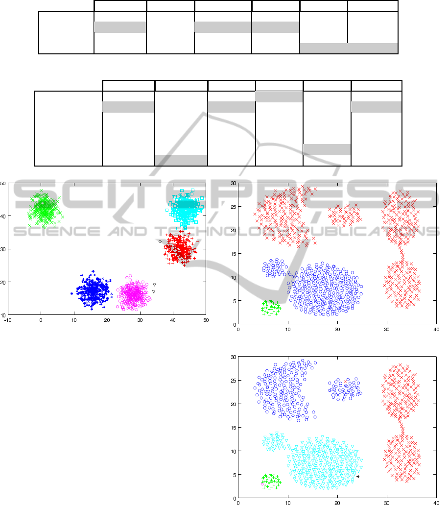
Table 4: Five groups data set validation results.
XB FS Kwon CWB PBM Silhouette
KMP (c=5) 7.64716 −540692 11494.1 0.608328 427.786 0.532795
FCM (c=5) 0.0506787 −523890 78.7023 0.155432 2101.97 0.730427
RAC 0.05887 −581968 91.0297 0.15704 3985.93 0.730427
HDA 0.0583695 −581594 90.1025 0.156968 4012.27 0.73118
Table 5: Aggregation data set validation results.
XB FS Kwon CWB PBM Silhouette
KMP (c=5&7) 0.320621 −86011.4 253.039 0.100997 98.4674 0.272249
FCM (c=5) 0.185912 −78942.4 148.601 0.215287 117.716 0.500565
FCM (c=7) 0.26758 −73294.5 214.788 0.34196 66.6775 0.467089
RAC − − − − − −
HDA (K=2.0) 1.98674 −128690 1567.92 0.329051 142.117 0.241994
HDA (K=0.7) 0.489475 −121270 387.897 0.295478 302.46 0.468173
HDA (K=0.8) 0.723013 −138778 571.038 0.310896 284.03 0.455008
Figure 6: Clustering result on five groups data set.
and the remaining five clusters then correspond to the
expected result. Table 4 shows the validation results
of our method and the compared methods for the five
groups data set. The results for the proposed method
were calculated after removing all outliers. Similarly
to the Iris data set, our method outperforms the other
hard clustering methods in the XB and Kwon indices
as well as in the CWB index for this data set. Our
method also produced the best values for the PBM
and Silhouette indices.
4.2.5 Aggregation Data Set
Fig. 7 shows the result of clustering the Aggregation
data set with our method. We can observe that the
three clusters produced are not ideal. The top 3 clus-
ters have been grouped together yet should be sep-
arate. After adjusting the merging constant K from
its default value of 2.0 to 0.8, we obtain the clustering
seen in fig. 8. This new clustering is better but still not
perfect as the upper-left and upper-center clusters are
still grouped together and some outliers are produced.
Figure 7: Clustering result on Aggregation data set.
Figure 8: Clustering result on Aggregation data set.
Reducing K to 0.7 produced the clustering seen in fig.
9. Reducing K further produced no improvement as
the clusterings produced were under-merged and rep-
resented the data even more poorly.
Table 5 shows the validation results of our method
and the compared methods for the Aggregation data
ICAART2014-InternationalConferenceonAgentsandArtificialIntelligence
208
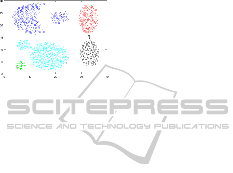
Figure 9: Clustering result on Aggregation data set.
set. The results for the proposed method were cal-
culated after removing all outliers. With the excep-
tion of the FS index, our method performed best with
a merging constant of 0.7. With these values, our
method outperformed the Y-means method in all but
the CWB index. For the other indices, our method
performed similarly but slightly worse than fuzzy c-
means with 5 clusters with the exception of the PBM
index where our method performed significantly bet-
ter. The RAC method has no values for this data set
as it clustered the entire data set into a single cluster.
5 CONCLUSIONS
In this paper, an automatic clustering method based
on a heuristic divisive approach has been proposed
and implemented. The method is based on the
DIANA algorithm interrupted by a heuristic stopping
function. As this process alone generally produces
too many clusters, its result is then passed on to a
merging method. The advantage of this two phase
approach being that with the splitting and merging us-
ing different criteria for determining if data belong in
a same cluster, the merged clusters can take non el-
liptical shapes. This advantage sets our method apart
from the majority of hard clustering methods in that it
can handle data which is not linearly separable fairly
well.
Five data sets have been used to evaluate the
proposed clustering method. The proposed method
was also compared against an automatic hard clus-
tering method, a fuzzy clustering method (for which
a known number of clusters was provided), and an
automatic clustering method based on fuzzy c-means
using multiple cluster validity indices. The proposed
method was shown to be roughly equivalent in effec-
tiveness as the others to which it was compared when
clustering linearly separable data sets and equivalent
or better when clustering non linearly separable data
sets without ever needing to be provided a number of
clusters.
There remains work to be done in finding more ap-
propriate validation methods to evaluate the proposed
method as the validity indices used fall victim to the
same pitfalls as most hard clustering methods when
the data set is not linearly separable. There also re-
mains to further optimize the proposed method and to
attempt modifying it for specific applications.
In conclusion, the proposed clustering method not
only identifies a desired number of clusters, but pro-
duces valid clustering results.
ACKNOWLEDGEMENTS
We gratefully acknowledge the support from NBIF’s
(RAI 2012-047) New Brunswick Innovation Funding
granted to Dr. Nabil Belacel.
REFERENCES
Bezdek, J. C., Ehrlich, R., and Full, W. (1984). Fcm: The
fuzzy c-means clustering algorithm. Computers &
Geosciences, 10(23):191–203.
Fisher, R. A. (1936). The use of multiple measurements in
taxonomic problems. Annals of Eugenics, 7(2):179–
188.
Fukuyama, Y. and Sugeno, M. (1989). A new method
of choosing the number of clusters for the fuzzy c-
means method. In Proceedings of Fifth Fuzzy Systems
Symposium, pages 247–250.
Gan, G. (2011). Data Clustering in C++: An Object-
Oriented Approach. Chapman and Hall/CRC.
Gionis, A., Mannila, H., and Tsaparas, P. (2007). Clustering
aggregation. ACM Trans. Knowl. Discov. Data, 1(1).
Guan, Y., Ghorbani, A., and Belacel, N. (2003). Y-
means: a clustering method for intrusion detection.
In Electrical and Computer Engineering, 2003. IEEE
CCECE 2003. Canadian Conference on, volume 2,
pages 1083–1086. IEEE.
Jain, A. K., Murty, M. N., and Flynn, P. J. (1999). Data
clustering: a review. ACM Comput. Surv., 31(3):264–
323.
Kaufman, L. R. and Rousseeuw, P. (1990). Finding groups
in data: An introduction to cluster analysis.
MacNaughton-Smith, P. (1964). Dissimilarity Analysis: a
new Technique of Hierarchical Sub-division. Nature,
202:1034–1035.
Mok, P., Huang, H., Kwok, Y., and Au, J. (2012). A
robust adaptive clustering analysis method for auto-
matic identification of clusters. Pattern Recognition,
45(8):3017–3033.
AHierarchicalClusteringBasedHeuristicforAutomaticClustering
209

Pakhira, M. K., Bandyopadhyay, S., and Maulik, U. (2004).
Validity index for crisp and fuzzy clusters. Pattern
Recognition, 37(3):487–501.
Pal, N. and Bezdek, J. (1995). On cluster validity for
the fuzzy c-means model. Fuzzy Systems, IEEE
Transactions on, 3(3):370–379.
Rezaee, M. R., Lelieveldt, B., and Reiber, J. (1998). A new
cluster validity index for the fuzzy c-mean. Pattern
Recognition Letters, 19(34):237–246.
Rousseeuw, P. J. (1987). Silhouettes: A graphical aid to
the interpretation and validation of cluster analysis.
Journal of Computational and Applied Mathematics,
20(0):53–65.
Wu, K.-L. and Yang, M.-S. (2005). A cluster validity in-
dex for fuzzy clustering. Pattern Recognition Letters,
26(9):1275–1291.
Xie, X. and Beni, G. (1991). A validity measure for fuzzy
clustering. Pattern Analysis and Machine Intelligence,
IEEE Transactions on, 13(8):841–847.
ICAART2014-InternationalConferenceonAgentsandArtificialIntelligence
210
