Adaptive Noise Variance Identification in Vision-aided Motion
Estimation for UAVs
Fan Zhou
1
, Wei Zheng
1
and Zengfu Wang
2
1
Department of Automation, University of Science and Technology of China, Hefei, China
2
Institute of Intelligent Machines, Chinese Academy of Sciences, Hefei, China
Keywords:
Adaptive Noise Variance Identification, Vision Location, Motion Estimation, Kalman Filter.
Abstract:
Vision location methods have been widely used in the motion estimation of unmanned aerial vehicles (UAVs).
The noise of the vision location result is usually modeled as the white gaussian noise so that this result could
be utilized as the observation vector in the kalman filter to estimate the motion of the vehicle. Since the
noise of the vision location result is affected by external environment, the variance of the noise is uncertain.
However, in previous researches the variance is usually set as a fixed empirical value, which will lower the
accuracy of the motion estimation. In this paper, a novel adaptive noise variance identification (ANVI) method
is proposed, which utilizes the special kinematic property of the UAV for frequency analysis and adaptively
identify the variance of the noise. Then, the adaptively identified variance are used in the kalman filter for
accurate motion estimation. The performance of the proposed method is assessed by simulations and field
experiments on a quadrotor system. The results illustrate the effectiveness of the method.
1 INTRODUCTION
The UAVs have become more and more popular in
recent years because of their widely applications in
mobile missions such as surveillance, exploration
and recognition in different environments. A main
problem in applications of unmanned aerial vehicles
(UAVs) is the estimation of the motion of the system,
including 3D position and translational speed.
Many research works have been done in this field,
using various kinds of location sensors including GPS
(Yoo and Ahn, 2003), laser range sensors (Farhad
et al., 2011; Vasconcelos et al., 2010), doppler radars
(Whitcomb et al., 1999), ultrasonic sensors (Zhao and
Wang, 2012), etc. However, the factors of accuracy,
weight, cost, and applicable environment limit the ap-
plication of these sensors on aerial vehicles. Vision
sensors, with advantage in these aspects, therefore
have become a popular choice for providing location
results of the system (Mondrag´on et al., 2010).
The kalman filter model is widely used to obtain
accurate,fast updated and reliable motion estimation
of the UAV system (Zhao and Wang, 2012; Chatila
et al., 2008; Bosnak et al., 2012), which generally
consists of two equations: the observation equation
and the state equation. Results directly provided by
the vision location method are used to establish the
observation equation of the kalman filter, and mea-
surements from inertial sensors are usually used to
establish the state equation.
In the kalman filter, the variance of the noise is
needed for estimation. The variance of the noise of
inertial sensors is basically statical and could be ob-
tained from the hardware data sheet. However, in vi-
sion location methods, feature detecting and match-
ing component is usually included, whose accuracy
is obviously affected by external environment, such
as illumination, camera resolution, texture of environ-
ment, height of flight etc. Therefore, the variance of
the noise of vision location results is changeable and
simply setting an empirical parameter of it will prob-
ably lower the accuracy of the motion estimation.
In this article, some special kinematic properties
of the UAV system, which were barely utilized be-
fore, are observed and utilized for frequency analysis
of the position signal (or the trajectory) of the vehicle.
Derivation shows that the position signal have some
characteristic in the frequency domain which helps to
separate it from the noise and therefore the variance
of the noise could be identified.
The rest of the paper is organized as follows. Sec-
tion 2 introduces the entire system where the ANVI
method is applied, including the configuration of the
UAV system and the principle of the motion estima-
753
Zhou F., Zheng W. and Wang Z..
Adaptive Noise Variance Identification in Vision-aided Motion Estimation for UAVs.
DOI: 10.5220/0004921707530758
In Proceedings of the 3rd International Conference on Pattern Recognition Applications and Methods (ICPRAM-2014), pages 753-758
ISBN: 978-989-758-018-5
Copyright
c
 2014 SCITEPRESS (Science and Technology Publications, Lda.)

tion. Section 3 proposed the ANVI method detailedly.
Experiment and results are shown in section 4 which
verified the feasibility and performance of the pro-
posed method. Some conclusions are presented in
section 5.
2 SYSTEM INTRODUCTION
2.1 UAV System Configuration
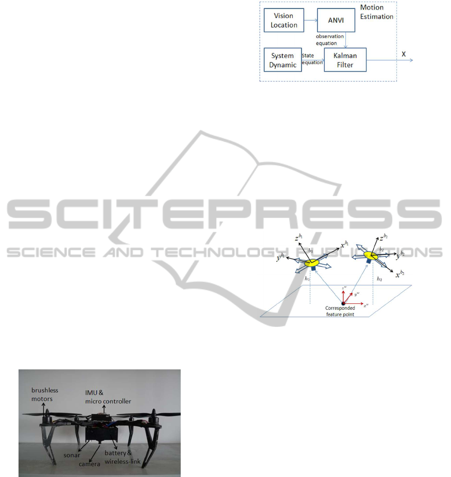
The configuration of our system is shown in Figure
1. The main sensors onboard is a downward looking
monocular camera, a height sensor and an IMU unit,
including an accelerometer, a gyroscope, and a mag-
netometer. The wireless link is used to share informa-
tion with the ground PC computer, where the vision
location algorithm is processing. An strap-down in-
ertial attitude estimation algorithm is executed on the
onboard micro controller. In the algorithm, the grav-
ity is measured by the 3-dimensional accelerometer,
which helps to establish the observation equation of
the attitude. Additionally, the angular velocity mea-
sured by the gyroscope helps to establish the propaga-
tion equation of the attitude. The two equations con-
stitute the kalman model for the attitude estimation.
Although we don’t discuss the attitude estimation in
this paper, some qualities of the attitude estimation
algorithm are indeed utilized for analysis of the posi-
tion signal of the system, which will be explained in
Section 3.1.
Figure 1: The configuration of the vehicle.
2.2 Principle of Motion Estimation
For automatical application, states of motion need to
be estimated, generally including 3D position p and
3D translational speed v, which form a 6-dimensional
state vector X = (p, v)
T
. Figure 2 shows the entire
framework of the states estimation in this paper. The
unique component of ANVI will be derived in Sec-
tion 3. The other components, as general parts of the
motion estimation, will be described in Section 2.
Figure 2: The framework of motion estimation.
2.2.1 Markless Vision Location
Figure 3 shows the environment of visual observa-
tion. The first frame captured by the camera is set
as the reference frame. Then, every frame captured
after will be compared with the reference frame. Af-
ter feature detecting and matching, which had been
widely studied in computer vision (R.Szeliski, 2010),
a location method could be presented with the pairs
of corresponded points.
Figure 3: Vision location.
As shown in Figure 3, the vehicle moved from lo-
cation 1 to location 2 (the attitude changed too), and
the related body frame are b
1
and b
2
, respectively. b
1
is where the reference video frame is captured. A
world coordinate frame is established with the center
point coincides with one of the corresponded feature
points p
w
0
= (x
w
0
, y
w
0
, z
w
0
)
T
.
With the knowledge of image formation process,
the coordinate of p
w
0
in the world frame could be
transformed into the coordinate in the image:
s
1


u
1
v
1
1


= M

R
1
t
1




x
w
0
y
w
0
z
w
0
1



(1)
Where (u
1
, v
1
)
T
denotes the coordinate in the im-
age. M denote the intrinsics matrix of the camera,
which could be obtained through calibration. R
1
and
t
1
denote the rotation and translation from the world
frame to the camera frame, respectively. In the ve-
hicle system, the rotation matrix R
1
could be ob-
tained by onboard strap-down inertial navigation sys-
tem (Savage, 1998; Edwan et al., 2011; de Marina
et al., 2012) so it could be treated as a known matrix.
ICPRAM2014-InternationalConferenceonPatternRecognitionApplicationsandMethods
754

s
1
is a scale factor. (x
w
0
, y
w
0
, z
w
0
)
T
denote the coordi-
nate of the feature point in the world frame. Since
the world frame is established with p
w
0
as the center
point, (x
w
0
, y
w
0
, z
w
0
)
T
= (0, 0, 0)
T
. Substituting it in (2),
one obtains
t
1
= s
1
M
−1


u
1
v
1
1


(2)
Another equation could be established with the
measurement of the height sensor:

R
−1
1
t
1

3
= h
1
(3)
Where the subscript 3 denotes the third element
of the vector. R
−1
1
is the inverse of R
1
and denotes
the rotation from the body frame to the world frame.
Obviously R
−1
1
t
1
is the location of the camera in the
world frame. h
1
is the measurement of the height sen-
sor.
Using (2) and (3), we have four equations with
four undetermined parameters (scale factor s
1
and
translation vector t
1
). The equations could be solved
and then the location of the camera in the world frame
p
w
c
1
could be represent as:
p
w
c
1
= R
−1
1
t
1
(4)
When the vehicle moved to location 2, as shown in
Figure 3, the location p
w
c
2
could be obtained with the
same equations presented above. Then, the relative
3D position between location 1 and 2 could be easily
calculated:
p = p
w
c
2
− p
w
c
1
(5)
The position result provided here by the vision lo-
cation method will be used as the observation vector
Z in the kalman filter. Note that this observation con-
tains noise, which is denoted as ξ and usually mod-
eled as the white gaussian noise. The variance of ξ is
needed in the kalman filter for estimation.
2.2.2 Dynamic of the System
The dynamic equation of the system motion is given
by
˙p
w
= v
w
˙v
w
= a
w
(6)
Where p
w
= (x
w
, y
w
, z
w
) denotes the position in the
world frame. v
w
, a
w
denotes the velocity and acceler-
ation in the world frame, respectively. Define R
w
b
as
the rotation matrix from the body frame to the world
frame. Then the acceleration in the world frame could
be obtained from
a
w
= R
w
b
a
b
a
b
= a
m
−n
a
−
−→
g
(7)
Substituting (7) into (6), one obtains the dynamic
model of the system:
˙p
w
= v
w
˙v
w
= R
w
b
(a
m
−n
a
−
−→
g )
(8)
Which could be transformed into discrete form:

p
w
v
w

k+1
=

1 ∆t
0 1

p
w
v
w

k
+

0
(R
w
b
a
m
k
−
−→
g )∆t

+

0
−R
w
b
n
a
∆t

(9)
Where ∆t denotes the update cycle of the ac-
celerometer.
2.2.3 Kalman Filter Model of the System
A popular model to fuse information from multiple
sensors is the kalman filter model, which consists of
a state equation and an observation equation. The vi-
sion location results helps to establish the observation
equation and the dynamic model helps to establish the
state equation. A classic kalman filter model is estab-
lished combining these two equations:

























"
p
w
v
w
#
k+1
=
"
1 ∆t
0 1
#"
p
w
v
w
#
k
+
"
0
(R
w
b
a
m
k
−
−→
g )∆t
#
+
"
0
−R
w
b
n
a
∆t
#
Z
k
=
h
1 0
i
"
p
w
v
w
#
k
+ ξ
k
(10)
Where X = (p
w
, v
w
)
T
denotes the state vector to
be estimated. The observation vector Z
k
is the vision
location result obtained in Section 2.2.1. ξ is the white
gaussian noise of the observation. In the kalman filter,
the variance of the noise is needed for processing. De-
fine Q
ξ
as the variance of ξ. Since the accuracy of the
vision location algorithm strongly depends on exter-
nal environment, Q
ξ
needs to be adaptively identified
to improve the accuracy of estimation.
AdaptiveNoiseVarianceIdentificationinVision-aidedMotionEstimationforUAVs
755

3 ADAPTIVE NOISE VARIANCE
IDENTIFICATION
The discrete observation signal Z(k) is provided by
the vision location algorithm at every 150ms. It con-
sists of the real position signal p(k) and the white
gaussian noise ξ(k).
Z(k) = p(k) + ξ(k) (11)
3.1 Characteristic of the Position Signal
in the Frequency Domain
To simplify the derivation, we first analyze p(t) in-
stead of p(k), which is the continuous form of the po-
sition.
Before the derivation of the characteristic of p(t)
in the frequency domain, some kinematic properties
of the vehicle need to be explained. That is, the mag-
nitude of the kinematic acceleration of the vehicle is
upper limited.
On one hand, acceleration with a certain upper
limit is enough for the vehicle to accomplish most of
the automatical missions. On the other hand, limit of
acceleration is actually a necessary condition for ac-
curate attitude estimation. It is easy to understander
that the kinematic acceleration will disturb the atti-
tude algorithm which uses the gravity for attitude es-
timation. The larger the acceleration of the vehicle is,
the less accurate the attitude estimation result will be,
which was detailedly explained in (de Marina et al.,
2012). Generally, by setting a upper limit of the throt-
tle, the roll angle and the pitch angle of the vehicle,
the acceleration is limited to:
|a| < 0.2g (12)
Now the position signal p(t) will be transformed
from the time domain to the frequency domain by the
Short-time Fourier transform (STFT). The speed sig-
nal v(t) and the acceleration signal a(t) will be used
in the following derivation, so they are also processed
here.
First, in the STFT, signals need to be intercepted
with a window. As shown in figure 4, ea(t), ev(t) and
ep(t) denote the signal intercepted from a(t), v(t) and
p(t) from t
1
to t
2
, respectively.
According to kinematic laws, the relation ship be-
tween ea(t), ev(t) and ep(t) is described in equation (13):
ep(t) =
Z
t
−∞
ev(t)dt + p
1
(u(t
1
−u(t
2
)))
ev(t) =
Z
t
−∞
ea(t)dt + v
1
(u(t
1
−u(t
2
)))
(13)
Figure 4: Interception of signals.
Where v
1
and p
1
denote the initial speed and po-
sition at time t
1
. u(t) denotes the unit step function.
Then, using qualities of the Fourier transform
(FT), one obtains
e
P( jω) =
e
V( jω)
jω
+ p
1
·G( jω)
= −
e
A( jω)
ω
2
+ (p
1
+
v
1
jω
) ·G( jω)
where
G( jω) =
r
π
2
(e
−jωt
1
−e
−jωt
2
)(
1
jωπ
+ δ(ω))
(14)
Where
e
P( jω),
e
V( jω) and
e
A( jω) denote the FT of
ep(t), ev(t) and ea(t), or the STFT of p(t), v(t) and a(t)
respectively. δ(ω) denotes the unit impulse function.
According to (12),



e
A( jω)



=




Z
t
2
t
1
ea(t)e
−jwt
dt




< 0.2g·(t
2
−t
1
) (15)
Therefore, according to (14) and (15)



e
P( jω)



<





e
A( jω)
ω
2





+




(p
1
+
v
1
jω
) ·G( jω)




<




0.2g·(t
2
−t
1
)
ω
2




+




(p
1
+
v
1
jω
)




·




√
2π(
1
jωπ
+ δ(ω))




(16)
Before practical STFT processing of the position
signal, the signal could be shifted so that the initial
value p
1
= 0, this won’t affecting the reconstruction
of the signal in the time domain. Therefore we obtain



e
P( jω)



<




0.2g·(t
1
−t
2
)
ω
2




+



v
1
ω



·




√
2π(
1
jωπ
+ δ(ω))




(17)
ICPRAM2014-InternationalConferenceonPatternRecognitionApplicationsandMethods
756

Equation (16) indicates the energy of the position
signal in the frequencydomain mostly distribute at the
low frequency part. To make it quantitative, we col-
lected sufficient position data during daily flight for
frequency analysis experiment, and the results con-
firmed the conclusion and indicated that the energy of
the position signal mostly distribute below 2Hz.
3.2 Identification of the Variance
According to the analysis in Section 3.1, we can Se-
lect a FIR bandpass digital filter H( jω), whose pass
band is above 2Hz. Let h(k) denotes the unit impulse
response of the FIR filter H( jω), whose length is n.
When we let the observation signal Z(k) through this
filter, the position signal p(k) will be filtered out, the
result signal is affected only by the noise signal ξ(k):
n−1
∑
k=0
(h(k) ·Z(k + k
0
))
=
n−1
∑
k=0
(h(k) ·(p(k + k
0
) + ξ(k+ k
0
)))
=
n−1
∑
k=0
(h(k) ·ξ(k+ k
0
))
(18)
Where k
0
denotes the start of the signal sequence.
As explained above, ξ(k) is the white gaussian noise,
so
E{ξ(k
1
) ·ξ(k
2
)} =
(
Q
ξ
, k
1
= k
2
0, k
1
6= k
2
(19)
Where E{·} denote the expected value of the sig-
nal.
Therefore
E{(
n−1
∑
k=0
(h(k) ·Z(k + k
0
)))
2
}
=E{(
n−1
∑
k=0
(h(k) ·ξ(k+ k
0
)))
2
}
=E{
n−1
∑
k=0
(h
2
(k) ·ξ
2
(k+ k
0
))}
=Q
ξ
·
n−1
∑
k=0
h
2
(k)
(20)
Therefore, we could obtain Q
ξ
from:
Q
ξ
=
E{(
∑
n−1
k=0
(h(k) ·Z(k + k
0
)))
2
}
∑
n−1
k=0
h
2
(k)
(21)
Where
∑
n−1
k=0
h
2
(k) is a known value when we se-
lected a known digital filter. (
∑
n−1
k=0
(h(k)·Z(k+ k
0
)))
2
is the Square of the the filtered result, which could
be calculated. The expected value of the filtered re-
sult E{(
∑
n−1
k=0
(h(k) ·Z(k + k
0
)))
2
} could be estimated
by average a length of sample data. The length of
the sample data is empirically selected. In practical,
when the length is selected longer, the estimation of
the expected value will be more accurate, but causes
heavier computation burden.
4 EXPERIMENTS AND RESULTS
4.1 Simulation of Adaptive Noise
Variance Identification
To verify the effectiveness of the ANVI method, we
plus the position signal provided by the assistant vi-
sual system with white gaussian noise whose variance
is known. The position signalwas mixed with dif-
ferent kinds of white gaussian noise whose variance
were 5cm, 10cm, 15cm and 20cm, respectively. Fig-
ure 5 shows the estimation result of the variance with
the proposed method, which is reliable and this result
is practical for further motion estimation.
Figure 5: Simulation: identification of the variance.
In practical application, the variance of the noise
generally changes not very fast. So to lower the com-
putational burden of the system, the estimation of the
variance is not executed every data sample cycle as
shown in Figure 5, but every 5-10 seconds.
4.2 Improvement of the Motion
Estimation
The identified variance Q
ξ
of the observation noise
is then used in the motion estimation based on the
kalman filter model in equation (10). The results of
AdaptiveNoiseVarianceIdentificationinVision-aidedMotionEstimationforUAVs
757

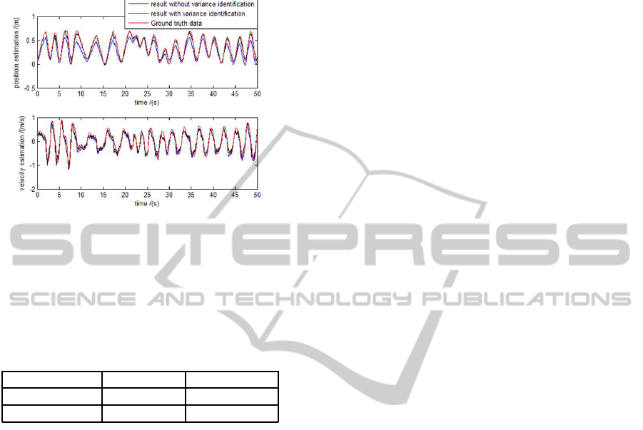
the motion estimation with a fixed empiric variance
value and with the ANVI method are recorded for
comparison.
Figure 6: Result of the motion estimation.
As shown in Figure 6, motion estimation includes
position estimation and velocity estimation, and the
accuracy of both improved with the ANVI method.
The root-mean-square error of the results compared
with the groudtruth data is shown in Table 1.
Table 1: Root-mean-square error of the results in Figure 7.
RMS error position(m) velocity(m/s)
without ANVI 0.110 0.151
with ANVI 0.037 0.105
5 CONCLUSIONS
A novel adaptive variance identification method is
proposed in this paper. Experiment shows that with
this method, variance of the noise could be identified
reliably. With the ANVI method, results of the motion
estimation will basically be optimal.
The method is especially suitable in the vision-
aided motion estimation of UAVs. Because firstly,
the noise of vision location results is changeable and
needs adaptive identification. Secondly, the validity
of the ANVI method is based on the special kinematic
properties of UAVs, as explained in the derivation.
However, since most kinds of robot share the same
kinematic properties that the kinematic acceleration
has a upper limit. Therefore, with certain adjustments
of the parameters, the proposed method could be used
in wide applications.
ACKNOWLEDGEMENTS
The work in this paper was supported by the Na-
tional Science and Technology Major Projects of the
Ministry of Science and Technology of China: ITER
(No.2012GB102007).
REFERENCES
Bosnak, M., Matko, D., and Blazic, S. (2012). Quadro-
copter hovering using position-estimation information
from inertial sensors and a high-delay video system.
Journal of Intelligent & Robotic Systems, 67(1):43–
60.
Chatila, R., Kelly, A., and Merlet, J, P. (2008). Hovering
flight and vertical landing control of a vtol unmanned
aerial vehicle using optical flow. In IEEE/RSJ IROS,
pages 801–806. IEEE.
de Marina, H, G., Pereda, F, J., Giron-Sierra, J, M., and
Espinosa, F. (2012). Uav attitude estimation using un-
scented kalman filter and triad. IEEE Transactions on
Industial Electronics, 59(11):4465–4474.
Edwan, E., Zhang, J, Y., and Zhou, J, C. (2011). Reduced
dcm based attitude estimation using low-cost imu and
magnetometer triad. In Proceedings of the 8th WPNC,
pages 1–6. IEEE.
Farhad, A., Marcin, K., and Galina, O. (2011). Fault-
tolerant position/attitude estimation of free-floating
space objects using a laser range sensor. IEEE Sen-
sors Journal, 11(1):176–185.
Mondrag´on, I., Olivares-M´endez, M., Campoy, P.,
Mart´ınez, C., and Mejias, L. (2010). Unmanned aerial
vehicles uavs attitude, height, motion estimation and
control using visual systems. Autonomous Robots,
29:17–34.
R.Szeliski (2010). Computer Vision: Algorithms and Appli-
cations. Springer, USA, 1nd edition.
Savage, P, G. (1998). Strapdown inertial navigation in-
tegration algorithm design part 1: attitude algo-
rithms. Journal of Guidance, Control, and Dynamics,
21(1):19–28.
Vasconcelos, J, F., Silvestre, C., and Oliveira, P. (2010).
Embedded uav model and laser aiding techniques
for inertial navigation systems. Control Engineering
Practice, 18(3):262–278.
Whitcomb, L., Yoerger, D., and Singh, H. (1999). Advances
in doppler-based navigation of underwater robotic ve-
hicles. In Proceedings of ICRA, volume 1, pages 399–
406. IEEE.
Yoo, C, S. and Ahn, I, K. (2003). Low cost gps/ins sensor
fusion system for uav navigation. In Proceedings of
the 22nd DASC, volume 2, pages 8.A.1–8.1–9. IEEE.
Zhao, H. and Wang, Z, Y. (2012). Motion measurement
using inertial sensors, ultrasonic sensors, and magne-
tometers with extended kalman filter for data fusion.
IEEE Sensors Journal, 12(5):943–953.
ICPRAM2014-InternationalConferenceonPatternRecognitionApplicationsandMethods
758