One-Step or Two-Step Optimization and the Overfitting Phenomenon

A Case Study on Time Series Classification

Muhammad Marwan Muhammad Fuad

Forskningsparken 3, Institutt for kjemi, NorStruct

The University of Tromsø - The Arctic University of Norway, NO-9037 Tromsø, Norway

Keywords: Bio-inspired Optimization, Differential Evolution, Overfitting, Time Series Classification.

Abstract: For the last few decades, optimization has been developing at a fast rate. Bio-inspired optimization

algorithms are metaheuristics inspired by nature. These algorithms have been applied to solve different

problems in engineering, economics, and other domains. Bio-inspired algorithms have also been applied in

different branches of information technology such as networking and software engineering. Time series data

mining is a field of information technology that has its share of these applications too. In previous works we

showed how bio-inspired algorithms such as the genetic algorithms and differential evolution can be used to

find the locations of the breakpoints used in the symbolic aggregate approximation of time series

representation, and in another work we showed how we can utilize the particle swarm optimization, one of

the famous bio-inspired algorithms, to set weights to the different segments in the symbolic aggregate

approximation representation. In this paper we present, in two different approaches, a new meta

optimization process that produces optimal locations of the breakpoints in addition to optimal weights of the

segments. The experiments of time series classification task that we conducted show an interesting example

of how the overfitting phenomenon, a frequently encountered problem in data mining which happens when

the model overfits the training set, can interfere in the optimization process and hide the superior

performance of an optimization algorithm.

1 INTRODUCTION

For the last few decades, optimization has been

developing at a fast rate. Novel algorithms appear

and new applications emerge in different fields of

engineering, economics, and science. The purpose of

an optimization process is to find the best-suited

solution of a problem subject to given constraints.

These constraints can be in the boundaries of the

parameters controlling the optimization problem, or

in the function to be optimized. This can be

expressed mathematically as follows: Let



nbp21

x,...,x,xX 

be the candidate solution to the

problem for which we are searching an optimal

solution. Given a function

RR 

nbp

U:f (nbp

is the number of parameters), find the solution



nbp

x,...,x,xX 

which satisfies:



UX,XfXf















The function f is called

the

fitness function, or the objective function (These

Figure 1: Some of the main bio-inspired metaheuristics.

two concepts are not really identical, but in this

paper we will use them interchangeably).

Metaheuristics

are probabilistic optimization

Bio-inspired Optimization

Swarm Intelligence

Evolutionary Algorithms

Genetic Algorithms

Differential Evolution

Genetic Programming

Evolution Strategies

Particle Swarm Optimization

Artificial Ant Colony

Artificial Bee Colony

645

Muhammad Fuad M..

One-Step or Two-Step Optimization and the Overﬁtting Phenomenon - A Case Study on Time Series Classiﬁcation.

DOI: 10.5220/0004916706450650

In Proceedings of the 6th International Conference on Agents and Artiﬁcial Intelligence (ICAART-2014), pages 645-650

ISBN: 978-989-758-015-4

 2014 SCITEPRESS (Science and Technology Publications, Lda.)

algorithms which are applicable to a large variety of

optimization problems. Metaheuristics can be

divided into

single solution –based metaheuristics

and population-based metaheuristics. Many of these

metaheuristics are inspired by natural processes,

natural phenomena, or by the collective intelligence

of natural agents, hence the term

bio-inspired, also

called nature-inspired, optimization algorithms.

Figure 1 shows the main bio-inspired metaheuristics.

One of the main bio-inspired optimization

families is

Evolutionary Algorithms (EA). EA are

population-based metaheuristics that use the

mechanisms of Darwinian evolution. The

Genetic

Algorithm

(GA) is the main member of EA. GA is

an optimization and search technique based on the

principles of genetics and natural selection (Haupt

and Haupt, 2004). GA has the following elements: a

population of individuals, selection according to

fitness, crossover to produce new offspring, and

random mutation of new offspring (Mitchell, 1996).

Differential Evolution (DE) is an optimization

method which is mainly effective to solve

continuous problems. DE is also based on the

principles of genetics and natural selection.

DE has the same elements as a standard

evolutionary algorithm; i.e. a population of

individuals, selection according to fitness, crossover,

and random mutation. DE starts with a collection of

randomly chosen individuals constituting a

population whose size is

popsize. Each of these

solutions is a vector of

nbp dimensions and it

represents a possible solution to the problem at hand.

The fitness function of each individual is evaluated.

The next step is optimization. In this step for each

individual, which we call the

target vector



, of the

population three mutually distinct individuals



, and different from



, are chosen at

random from the population. The

donor vector D



formed as a weighted difference of two of



added to the third; i.e.





321 rrr

VVFVD



 .

is called the mutation

factor

or the differentiation constant and it is one of

the control parameters of DE.

The

trial vector R



is formed from elements of

the target vector



and elements of the donor

vector



. In the following we present the crossover

scheme presented in (Feoktistov, 2006) which we

adopt in this paper; an integer

Rnd is randomly

chosen among the dimensions



nbp,1 . Then the trial

vector



is formed as follows:

























otherwise

iRndC1,0randif

ttFt

j,i

rj,i

3r,i2r,i1r,i

(1)

where

nbp,...,i 1



C is the crossover constant,

which is another control parameter.

The next step of DE is selection. This step

decides which of the trial vector and the target

vector will survive in the next generation and which

will die out. The selection is based on which of the

two vectors; trial and target, yields a better value of

the fitness function. Crossover and selection repeat

for a certain number of generations.

□

Data mining is a field of computer science which

handles several tasks such as classification,

clustering, anomaly detection, and others.

Processing these tasks usually requires extensive

computing. As with other fields of computer science,

different papers have proposed applying bio-inspired

optimization to data mining tasks (Muhammad Fuad,

2012a, 2012b, 2012c, 2012d).

Data mining models may suffer from what is

called

overfitting. A classification algorithm is said

overfit to the training data if it generates a

representation of the data that depends too much on

irrelevant features of the training instances, with the

result that it performs well on the training data but

relatively poorly on unseen instances (Bramer,

2007). In overfitting the algorithm memorizes the

training set at the expense of generalizability to the

validation set (Larose, 2005).

We will show in this paper a generalization of

the optimization methods that we presented in

(Muhammad Fuad, 2012b, 2012c, 2012d) and how

the overfitting phenomenon can interfere to alter the

outcome of the optimization process. In Section 2

we present the problem and our previous work on it

and the new generalization, in two different

approaches, of this previous work. We compare

these two approaches in Section 3 and we discuss

the results of the experiments in Section 4. We

conclude the paper in Section 5.

ICAART2014-InternationalConferenceonAgentsandArtificialIntelligence

646

2 ONE-STEP OR TWO-STEP

OPTIMIZATION OF THE

SYMBOLIC AGGREGATE

APPROXIMATION

A time series S is an ordered collection:

  

nn2211

v,t,...,v,t,v,tS 

(2)

where

n21

t...tt  , and where

v are the values

of the observed phenomenon at time points

t .

Time series data mining handles several tasks

such as classification, clustering, similarity search,

motif discovery, anomaly detection, and others.

Time series are high-dimensional data so they

are usually processed by using representation

methods that are used to extract features from these

data and project them on lower-dimensional spaces.

The

Symbolic Aggregate approXimation method

(SAX) (Lin et. al., 2003) is one of the most

important representation methods of time series. The

main advantage of SAX is that the similarity

measure it uses, called MINDIST, uses statistical

lookup tables, which makes it easy to compute with

an overall complexity of



NO . SAX is based on

the assumption that normalized time series have

Gaussian distribution, so by determining the

breakpoints that correspond to a particular alphabet

size, one can obtain equal-sized areas under the

Gaussian curve. SAX is applied as follows:

1-The time series are normalized.

2-The dimensionality of the time series is reduced

using PAA (Keogh

et. al., 2000), (Yi and Faloutsos,

2000).

3-The PAA representation of the time series is

discretized by determining the number and location

of the breakpoints (The number of the breakpoints is

chosen by the user). Their locations are determined,

as mentioned above, using Gaussian lookup tables.

The interval between two successive breakpoints is

assigned to a symbol of the alphabet, and each

segment of PAA that lies within that interval is

discretized by that symbol.

The last step of SAX is using the following

similarity measure:











dist

MINDIST

(3)

Where

is the length of the original time series,

N is the length of the strings (the number of the

segments),

and R

are the symbolic representations

of the two time series

and

, respectively, and

where the function

)(dist is implemented by using

the appropriate lookup table. It is proven that the

similarity measure in (3) produces no false

dismissals.

In (Muhammad Fuad, 2012b), (Muhammad

Fuad, 2012c), we showed that this assumption of

Gaussianity oversimplifies the problem and can

result in very large errors in time series mining

tasks, and we presented alternatives to SAX; one

which is based on the genetic algorithms (GASAX),

and another which is based on the differential

evolution (DESAX), to determine the locations of

the breakpoints. We showed that these two

optimized alternatives clearly outperform the

original SAX.

In (Muhammad Fuad, 2012d), we used

Particle

Swarm Optimization

(PSO), well-known

metaheuristics, to optimize SAX using a different

approach; to propose a new minimum distance

WMD that can better recover the information loss

resulting from SAX. The method we introduced,

(PSOWSAX), gives different weights to different

segments of the times series in the lower-

dimensional space. These weights are proportional

to the information contents of the different

segments. In (PSOWSAX) PSO is utilized to set

these weights.

□

A logical extension, which we present in this

work, of the above optimized alternatives to SAX is

one meta optimization process that can find optimal

locations of the breakpoints and optimal weights of

the segments corresponding to these breakpoints.

Such an optimization process can actually be

handled in two different ways; the first, which we

call

Two-Step OSAX constitutes of two steps, as the

name implies. In the first step the optimization

searches for the optimal locations of the breakpoints

assuming that all segments have the same weight

= 1

, and then in the next step another optimization

process sets optimal weights based on the optimal

locations of the breakpoints, which are the outcome

of step one. Since the weights are related to the

locations of the breakpoints, it is logical that step

one should start by optimizing the locations of the

breakpoints. The other way, which we call

One-Step

OSAX

uses one step to find the optimal locations of

the breakpoints and the weights corresponding to

those breakpoints.

We tended to think before conducting the

experiments that

Two-Step OSAX will give better

results than

One-Step OSAX since it seemed more

intuitive. We will see in the experimental section if

this intuition is founded.

One-SteporTwo-StepOptimizationandtheOverfittingPhenomenon-ACaseStudyonTimeSeriesClassification

647

3 EXPERIMENTS

We conducted the same experiments that we used to

validate (GESAX), (DESAX), and (PSOWSAX),

which are

1-NN classification task experiments. The

goal of classification, one of the main tasks of data

mining, is to assign an unknown object to one out of

a given number of classes, or categories (Last,

Kandel, and Bunke , 2004). In

k-NN each time

series is assigned a class label. Then a “leave one

out” prediction mechanism is applied to each time

series in turn; i.e. the class label of the chosen time

series is predicted to be the class label of its nearest

neighbor, defined based on the tested distance

function. If the prediction is correct, then it is a hit;

otherwise, it is a miss.

The classification error rate is defined as the ratio

of the number of misses to the total number of time

series (Chen and Ng, 2004).

1-NN is a special case

k-NN, where k=1.

We conducted experiments using datasets of

different sizes and dimensions available at UCR

(Keogh

et. al., 2011).

The values of the alphabet size we tested in the

experiments were 3, 10, and 20. We chose these

values because the first version of SAX used

alphabet size that varied between 3 and 10. Then in a

later version the alphabet size varied between 3 and

20. So these values are benchmark values.

As for the control parameters of DE that we

used, the population size

popsize was 12. The

differentiation constant F

was set to 0.9, and the

crossover constant C

was set to 0.5. The dimension

of the problem

nbp is breakpoints + weights in One-

Step OSAX

, and it is breakpoints and weights, in the

first step of

Two-Step OSAX and the second step of

Two-Step OSAX, respectively. As for the number of

generations NrGen, it is 100 for One-Step OSAX and

50 for each step of

Two-Step OSAX. Since the fitness

function is the same (the classification error) this

configuration guarantees that the complexities of

One-Step OSAX and that of Two-Step OSAX are

almost the same.

The training phase for

Two-Step OSAX is as

follows; for each value of the alphabet size, we run

the optimization process for 50 generations to get

the optimal locations of the breakpoints. This

corresponds to the first step of

Two-Step OSAX, then

we use these optimal locations of the breakpoints to

run the optimization process for 50 generations to

obtain the optimal weights. Later we use these

optimal weights and locations of the breakpoints on

the testing datasets to obtain the minimal

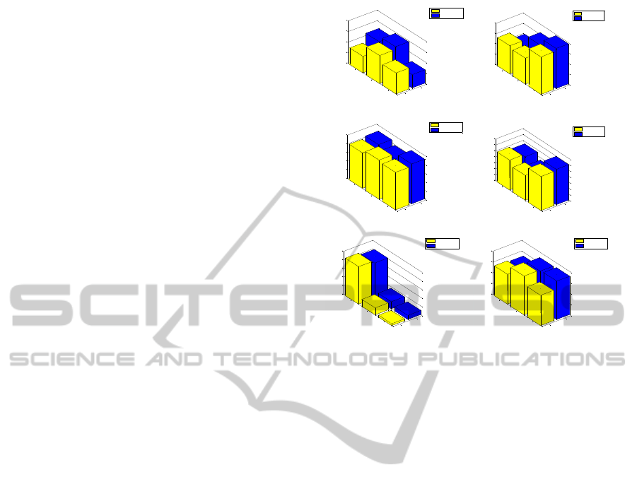
classification error (which we show in Figure 2 for

OneStepSA X

TwoStepSAX

0.05

0.1

0.15

0.2

DiatomSizeReduction

alphabet-size

Classification Error

OneStepSAX

TwoStepSAX

OneStepS AX

TwoStepSAX

0.05

0.1

0.15

0.2

FaceFour

alphabet-size

Classification Error

OneStepSAX

TwoStepSAX

OneStepSA X

TwoStepSAX

0.05

0.1

0.15

0.2

0.25

MoteStrain

alphabet-size

Classification Error

OneStepSAX

TwoStepSAX

OneStepS AX

TwoS te pS AX

0.05

0.1

0.15

0.2

0.25

0.3

0.35

SonyAIBORobotSurfaceII

alphabet-size

Classification Error

OneStepSAX

TwoStepSAX

OneStepSA X

TwoStepSAX

0.05

0.1

0.15

0.2

0.25

SyntheticControl

alphabet-size

Classification Error

OneStepSAX

TwoStepSAX

OneStepSA X

TwoStepSAX

0.1

0.2

0.3

0.4

TwoLeadECG

alphabet-size

Classification Error

OneStepSAX

TwoStepSAX

Figure 2: Comparison of the classification errors between

One-Step OSAX and Two-Step OSAX on different testing

datasets.

some of the different datasets that we tested in our

experiments). As for the experimental protocol for

One-Step OSAX, it is the same as that for Two-Step

OSAX

, except that we optimize in one step for the

locations of the breakpoints and for the weights, also

NrGen in the case is equal to 100.

The results shown in Figure 2 do not show, in

general, a difference in performance between

One-

Step OSAX

and Two-Step OSAX. We will discuss

these results more thoroughly in the next section.

4 DISCUSSION

At first glance the results we obtained in Section 3

suggest that there is no real difference between the

performance of

One-Step OSAX and that of Two-

Step OSAX

. We have to admit that these results were

a bit surprising to us as we expected, before

conducting the experiments, that

Two-Step OSAX

would give better results than those obtained by

applying

One-Step OSAX for reasons we mentioned

in Section 2. However, a deeper examination of the

results may yet reveal more surprising results.

If we remember from the experimental protocol

illustrated in the previous section, the two

optimization processes:

One-Step OSAX and Two-

Step OSAX

are applied to the training datasets to find

the optimal locations of the breakpoints and the

ICAART2014-InternationalConferenceonAgentsandArtificialIntelligence

648

Table 1: Comparison of the classification errors between One-Step OSAX and Two-Step OSAX on the training datasets

presented in Figure 2.

Dataset Method

Classification Error

=3 α=10 α=20

DiatomSizeReduction

One-Step OSAX

0.062 0.062 0.062

Two-Step OSAX

0.687 0.125 0.062

FaceFour

One-Step OSAX

0.042 0.042 0.167

Two-Step OSAX

0.292 0.167 0.167

MoteStrain

One-Step OSAX

0.150 0.050 0.050

Two-Step OSAX

0.700 0.150 0.100

SonyAIBORobotSurfaceII

One-Step OSAX

0.148 0.111 0.074

Two-Step OSAX

0.444 0.185 0.148

synthetic_control

One-Step OSAX

0.170 0.003 0.000

Two-Step OSAX

0.833 0.020 0.003

TwoLeadECG

One-Step OSAX

0.130 0.087 0.043

Two-Step OSAX

0.652 0.260 0.087

is the alphabet size

optimal weights, and then these optimal values are

applied to the testing datasets, so the real

comparison between the efficiency of

One-Step

OSAX

and Two-Step OSAX, as optimization

processes, should in fact compare their performances

on the training datasets. Table 1 shows the

classification error; the fitness function in our

optimization problem, obtained by applying

One-

Step OSAX

and Two-Step OSAX to the datasets

presented in Figure 2. The results presented in Table

1 show that

One-Step OSAX clearly outperforms

Two-Step OSAX. These results raise two questions;

the first is why these results did not appear in Figure

2, which represents the final outcome of the whole

process, and the second question is why

One-Step

OSAX

outperformed Two-Step OSAX. As for the first

and the most interesting question which is why the

superior performance of

One-Step OSAX did not

show in the final results presented in Figure 2, the

reason for this is that the optimal solutions obtained

One-Step OSAX on the training datasets

overfitted the data; they were “too good” that when

they were used on the testing datasets the

performance dropped. This was not the case with

Two-Step OSAX. This interesting finding may

establish a new strategy to applying optimization in

data mining that “less optimal” solutions obtained by

applying the optimization algorithm to the training

datasets may finally turn out to be better than “more

optimal” solutions which may overfit the training

data.

As for the other question of why

One-Step OSAX

outperformed Two-Step OSAX, we believe the

reason for this could be that finally the locations of

the breakpoints play a more important role in the

optimization process than the weights, so in

One-

Step OSAX

the optimization process kept improving

the locations of the breakpoints until the final stages

of the optimization process while

Two-Step OSAX

interrupted this optimization after the first step.

5 CONCLUSIONS

In this paper we presented two approaches of an

optimization algorithm that handles a certain

problem of time series classification. These time

series are represented using a symbolic

representation method, SAX, of time series data.

Our optimized versions produce optimal versions, in

terms of classification task accuracy, of the original

SAX in that they spot optimal locations of the

breakpoints and optimal weights compared with the

original SAX. The first of the two approaches we

presented,

One-Step OSAX, consists of one step to

perform the optimization process, while the second

one,

Two-Step OSAX, applies the optimization

process in two steps. The experiments we conducted

show that

One-Step OSAX outperforms Two-Step

OSAX

. The interesting finding of our experiments is

that the superior performance of One-Step OSAX

was actually “hidden” because of the overfitting

phenomenon.

We believe the results we obtained shed new

light on the application of optimization algorithms,

mainly stochastic and bio-inspired ones, in data

mining, where the risk of overfitting is frequently

present. We think that an optimization algorithm,

applied to the training data, should avoid searching

for very close-to-optimal solutions, which highly fit

the training data and thus may not give optimal

One-SteporTwo-StepOptimizationandtheOverfittingPhenomenon-ACaseStudyonTimeSeriesClassification

649

solutions when deployed to testing data. A possible

strategy that we suggest is to terminate the

optimization process, on the training sets,

prematurely. However, the output of our

experiments applies to times series only, and to the

classification task in particular, so we do not have

enough evidence that our remarks are generalizable.

REFERENCES

Bramer, M., 2007. Principles of Data Mining,

Undergraduate Topics in Computer Science, Springer.

Chen, L., Ng, R., 2004. On the Marriage of Lp-Norm and

Edit Distance, In Proceedings of 30th International

Conference on Very Large Data Base, Toronto,

Canada, August, 2004.

Feoktistov, V., 2006. Differential Evolution: “In Search of

Solutions” (Springer Optimization and Its

Applications)”. Secaucus, NJ, USA: Springer- Verlag

New York, Inc..

Haupt, R.L., Haupt, S. E., 2004. Practical Genetic

Algorithms with CD-ROM. Wiley-Interscience.

Keogh, E., Chakrabarti, K., Pazzani, M., and Mehrotra ,

2000. Dimensionality reduction for fast similarity

search in large time series databases. J. of Know. and

Inform. Sys.

Keogh, E., Zhu, Q., Hu, B., Hao. Y., Xi, X., Wei, L. &

Ratanamahatana, C.A., 2011. The UCR Time Series

Classification/Clustering Homepage: www.cs.ucr.edu/

~eamonn/time_series_data/

Larose, D., 2005. Discovering Knowledge in Data: An

Introduction to Data Mining, Wiley, Hoboken, NJ.

Last, M., Kandel, A., and Bunke, H., editors. 2004. Data

Mining in Time Series Databases. World Scientific.

Lin, J., Keogh, E., Lonardi, S., Chiu, B. Y., 2003. A

symbolic representation of time series, with

implications for streaming algorithms. DMKD 2003:

2-11.

Mitchell, M., 1996. An Introduction to Genetic

Algorithms, MIT Press, Cambridge, MA.

Muhammad Fuad, M.M., 2012a. ABC-SG: A New

Artificial Bee Colony Algorithm-Based Distance of

Sequential Data Using Sigma Grams. The Tenth

Australasian Data Mining Conference - AusDM 2012,

Sydney, Australia, 5-7 December, 2012. Published in

the CRPIT Series-Volume 134, pp 85-92.

Muhammad Fuad, M.M. , 2012b. Differential Evolution

versus Genetic Algorithms: Towards Symbolic

Aggregate Approximation of Non-normalized Time

Series. Sixteenth International Database Engineering

& Applications Symposium– IDEAS’12 , Prague,

Czech Republic,8-10 August, 2012 . Published by

BytePress/ACM.

Muhammad Fuad, M.M. , 2012c. Genetic Algorithms-

Based Symbolic Aggregate Approximation. 14th

International Conference on Data Warehousing and

Knowledge Discovery - DaWaK 2012 – Vienna,

Austria, September 3 – 7.

Muhammad Fuad, M.M. , 2012d. Particle Swarm

Optimization of Information-Content Weighting of

Symbolic Aggregate Approximation. The 8th

International Conference on Advanced Data Mining

and Applications -ADMA2012, 15-18 December 2012,

Nanjing, China . Published by Springer-Verlag in

Lecture Notes in Computer Science/Lecture Notes in

Artificial Intelligence, Volume 7713, pp 443-455.

Yi, B. K., and Faloutsos, C., 2000. Fast time sequence

indexing for arbitrary Lp norms. Proceedings of the

26th International Conference on Very Large

Databases, Cairo, Egypt.

ICAART2014-InternationalConferenceonAgentsandArtificialIntelligence

650