Reducing Sample Complexity in Reinforcement Learning by
Transferring Transition and Reward Probabilities
Kouta Oguni
1
, Kazuyuki Narisawa
1
and Ayumi Shinohara
1
1
Graduate School of Information Sciences, Tohoku University,
Aramaki aza Aoba 6-3-09, Aoba-ku, Sendai, Miyagi 980-8579, Japan
Keywords:
Reinforcement Learning, Transfer Learning, Sample Complexity, PAC-MDP.
Abstract:
Most existing reinforcement learning algorithms require many trials until they obtain optimal policies. In this
study, we apply transfer learning to reinforcement learning to realize greater efficiency. We propose a new
algorithm called TR-MAX, based on the R-MAX algorithm. TR-MAX transfers the transition and reward
probabilities from a source task to a target task as prior knowledge. We theoretically analyze the sample
complexity of TR-MAX. Moreover, we show that TR-MAX performs much better in practice than R-MAX in
maze tasks.
1 INTRODUCTION
Reinforcement learning is one of the useful meth-
ods for providing control rules for machines, where
an agent learns its own policy for an unknown envi-
ronment autonomously. Programmers do not have to
provide explicit rules for machines if the learning is
powerful enough. In reinforcement learning, learners
consume many trials until they obtain optimal rules,
however it is difficult in real world learning. Recent
studies (Tan, 1993; Miyazaki et al., 1997; Kretchmar.,
2002) have attempted to reduce the number of trials
for efficient learning.
Some researchers have applied transfer learning
to reinforcement learning (Konidaris and Barto, 2006;
Taylor and Stone, 2009; Taylor et al., 2007). Trans-
fer learning applies the knowledge obtained in some
source tasks to a target task to solve it efficiently.
Some studies (Konidaris and Barto, 2006; Taylor
et al., 2007) experimentally showed that applying
transfer learning to reinforcement learning is effective
in reducing the number of trials.
However, the theoretical aspects of transfer learn-
ing for reinforcement learning are not yet fully
known. In (Mann and Choe, 2012), the authors de-
fined an α-weak admissible heuristic and showed the-
oretically that transferring some action values yields
efficient reinforcement learning.
In this position paper, we outline our approach to
transfer learning for reinforcement learning: we try to
transfer the transition probability and reward proba-
bility as knowledge, because they should be useful for
efficient learning.
On the basis of the theoretical framework in
(Kakade, 2003; Strehl and Littman, 2005) we pro-
pose the efficient learning algorithm TR-MAX that
is an extension of R-MAX (Brafman and Tennen-
holtz, 2003). From a theoretical viewpoint, we show
the sample complexity of TR-MAX, which is smaller
than that of R-MAX, and it implies that TR-MAX is
PAC-MDP (Kakade, 2003). From a practical view-
point, we compare TR-MAX with R-MAX in maze
problems and verify that our TR-MAX algorithm is
indeed efficient.
2 PRELIMINARIES
The reinforcement learning framework assumes that
its task satisfies the Markov property. This task is
called a Markov decision process (MDP) (Sutton and
Barto, 1998).
Definition 1. A finite Markov Decision Process is a
five tuple hS,A,T,R,γi. S is a finite set called the state
space, and A is a finite set called the action space.
T : S× A× S → [0,1] is the transition probability, and
R : S× A → R is the reward function. 0 ≤ γ < 1 is the
discount factor.
According to the related work (Strehl et al., 2009;
Mann and Choe, 2012), we assume that rewards take
a value in the interval [0,1], so that we obtain R : S×
632
Oguni K., Narisawa K. and Shinohara A..
Reducing Sample Complexity in Reinforcement Learning by Transferring Transition and Reward Probabilities.
DOI: 10.5220/0004915606320638
In Proceedings of the 6th International Conference on Agents and Artificial Intelligence (ICAART-2014), pages 632-638
ISBN: 978-989-758-015-4
Copyright
c
 2014 SCITEPRESS (Science and Technology Publications, Lda.)

A → [0, 1]. M denotes a finite MDP in the sequel.
Definition 2. For any policy in M, let
V
π
M
(s) = E
π
"
∞
∑
i=0
γ
i
r
t+1+i





s
t
= s
#
denote the policy (or state) value function from state
s
t
= s at timestep t, and let
Q
π
M
(s,a) = E
π
"
∞
∑
i=0
γ
i
r
t+1+i





s
t
= s,a
t
= a
#
denote the action value function from state s
t
= s
and action a
t
= a. Note that s
t
denotes the state at
timestep t, and a
t
denotes the action at timestep t.
The policy (or state) value function indicates how
good it is to be in a particular state for the agent.
Moreover, the action value function indicates how
good it is to perform the action in that state for the
agent.
A policy π
∗
is called optimal if it satisfies
V
π
∗
M
(s) ≥ V
π
M
(s) for any policy π and state s ∈ S.
Definition 3 ((Kakade, 2003)). Let (s
1
,a
1
,r
1
,
s
2
,a
2
,r
2
,...) be a random path generated by execut-
ing an algorithm A in an MDP M. For any fixed
ε > 0, the sample complexity of A is the number of
timesteps t such that the policy A
t
at time t satis-
fies V
A
t
M
(s
t
) < V
π
∗
M
(s
t
) − ε. The algorithm A is called
Probably Approximately Correct in Markov Decision
Processes (PAC-MDP) if the sample complexity of A
is bounded by some polynomial in |S|, |A|,
1
ε
,
1
δ
,
1
(1−γ)
with probability at least 1 − δ, for any 0 < ε < 1 and
0 < δ < 1.
If a reinforcement learning algorithm is PAC-
MDP, the algorithm can efficiently learn in any MDP.
Definition 4 ((Kakade, 2003)). Let (s
1
,a
1
,r
1
,
s
2
,a
2
,r
2
,...) be a random path generated by execut-
ing an algorithm A in an MDP M. For any fixed
ε > 0, the sample complexity of A is the number of
timesteps t such that the policy A
t
at time t satis-
fies V
A
t
M
(s
t
) < V
π
∗
M
(s
t
) − ε. The algorithm A is called
Probably Approximately Correct in Markov Decision
Processes (PAC-MDP) if the sample complexity of A
is bounded by some polynomial in |S|, |A|,
1
ε
,
1
δ
,
1
(1−γ)
with probability at least 1 − δ, for any 0 < ε < 1 and
0 < δ < 1.
If a reinforcement learning algorithm is PAC-
MDP, the algorithm can efficiently learn in any MDP.
Brafman et al. (Brafman and Tennenholtz, 2003)
proposed an efficient model based algorithm called
R-MAX
1
. Model-based algorithms maintain not
1
The R-MAX algorithm is obtained from Algorithm 1
by omitting lines 7-16, because our TR-MAX algorithm is
an extension of the R-MAX algorithm.
only the rewards but also the number of selections
select(s,a) and the number of transitions trans(s,a,s
′
)
for any state s,s
′
∈ S and action a ∈ A, and cal-
culate the empirical transition probability T(s
′
|s,a)
and the empirical expectation of the reward distri-
bution
ˆ
R(s,a). In R-MAX, the action value is up-
dated only for the state-action pairs (s,a) satisfying
select(s,a) ≥ m. The sample complexity of R-MAX
is analyzed by (Strehl et al., 2009) as follows.
Theorem 1 ((Strehl et al., 2009)). Let 0 < ε <
1
1−γ
and 0 < δ < 1 be any real numbers, and as-
sume that the two inputs m and ε
1
of R-MAX in
M satisfy m = O

|S| + ln
|S||A|
δ

X
2

where X =
V
max
/(ε(1 − γ)) and
1
ε
1
= O

1
ε

. Let A
t
denote the
policy of R-MAX at timestep t and s
t
denote the state
at timestep t. Then, V
A
t
M
(s
t
) ≥ V
∗
M
(s
t
) − ε is true for
all but
O

|S||A|

|S| + ln
|S||A|
δ

X
3
Y

,
where Y = ln
1
δ
ln
1
ε(1− γ)
timesteps t with probability at least 1− δ.
Corollary 1. R-MAX is PAC-MDP.
By corollary 1, in theory, R-MAX performs effi-
ciently for any MDP. In practice, however, it is very
slow compared with other well-known algorithms
such as Sarsa(λ) (Rummery and Niranjan, 1994), be-
cause R-MAX requires many trials in order to guar-
antee the theoretical bound for all states and actions.
We note that R-MAX uses no prior knowledge for the
reinforcement learning problem.
3 TR-MAX
In this section, we propose the learning algorithm TR-
MAX, which uses prior knowledge in order to speed
up learning.
First, we define a heuristic transition function
T
h
: S× A× S → [0,1] and a heuristic reward function
R
h
: S× A → [0,1]. They are regarded as prior knowl-
edge of M. Next, we define the useful knowledge for
efficient reinforcement learning.
Definition 5. For a state-action pair (s, a) ∈ S × A,
we define the set Z
s,a
⊂ S of zero-transitioned states
by
Z
s,a
:=

s
′
∈ S | T(s
′
|s,a) = T
h
(s
′
|s,a) = 0

.
This means that the agent never transitions to any
s
′
∈ Z
s,a
from state s by action a, and this fact is
ReducingSampleComplexityinReinforcementLearningby
TransferringTransitionandRewardProbabilities
633

known to the agent via T
h
. We simply denote |Z
min
| =
min
(s,a)∈S×A
|Z
s,a
| in the sequel.
Definition 6. Let M be a finite MDP whose optimal
action value is upper bounded by V
max
, and T
h
(resp.
R
h
) be a heuristic transition (resp. reward) function
for M. For any 0 < ε <
1
1−γ
, we define the set P
ε
⊂
S× A of useful state-action pairs by
P
ε
:=

(s,a) ∈ S × A



|R(s,a) − R
h
(s,a)| ≤
ε(1− γ)
V
max
,
∑
¯s∈S


T( ¯s|s,a) − T
′
( ¯s|s,a)


≤
ε(1− γ)
V
max
)
.
This means that the heuristic values provided by T
h
and R
h
are close enough to the true probabilities for
the state-action pairs (s,a) ∈ P
ε
.
Algorithm 1 describes our algorithm TR-MAX,
which is based on R-MAX: the input arguments
T
h
, R
h
, Z and P
ε
, and lines 7-16 are added to R-
MAX, to utilize the prior knowledge for M;
ˆ
T(s
′
|s,a)
and
ˆ
R(s,a) are initialized by using T
h
(s
′
|s,a) and
R
h
(s,a) respectively if they are useful (lines 7-13);
and Q(s,a) is initialized to reflect them (lines 14-
16). Most model-based algorithms consume a con-
siderable number of timesteps to make the empiri-
cal probabilities close to the true probabilities for all
pairs (s,a) ∈ S×A, whereas TR-MAX does it only for
(s,a) /∈ P
ε
, owing to the prior knowledge. We show
the sample complexity of TR-MAX as follows.
Theorem 2. Let 0 < ε <
1
1−γ
and 0 < δ < 1 be
any real numbers, and T
h
(reps. R
h
) be a heuris-
tic transition (resp. reward ) function for M. Sup-
pose that two inputs m and ε
1
of TR-MAX in
M satisfy m = O

|S| − |Z
min
| + ln
|S||A| − |P
ε
|
δ

X
2

,
where X = V
max
/(ε(1 − γ)), and
1
ε
1
= O

1
ε

. Then,
V
A
t
M
(s
t
) ≥ V
∗
M
(s
t
) − ε is true for all but
O

(|S||A| − |P
ε
|)

|S| − |Z
min
| + ln
|S||A| − |P
ε
|
δ

X
3
Y

,(1)
where Y = ln
1
δ
ln
1
ε(1− γ)
timesteps t with probability at least 1− δ.
As a special case, if T(s
′
|s,a) = T
h
(s
′
|s,a) holds
for all (s,a,s
′
) ∈ S × A× S, then V
A
t
M
(s
t
) ≥ V
∗
M
(s
t
) − ε
is true for all but
O

(|S||A| − |P
ε
|)ln
|S||A| − |P
ε
|
δ
X
3
Y

(2)
timesteps t with probability at least 1− δ.
By Theorem 2, the sample complexity of TR-
MAX is less than that of R-MAX if either |Z
min
| or
Algorithm 1: TR-MAX.
Input: S, A, γ,m, ε
1
,T
h
,R
h
,Z and P
ε
1 forall the (s, a) ∈ S× A do
2 Q(s,a) ←
1
1−γ
; select(s,a) ← 0;
3 forall s
′
∈ S do trans(s,a, s
′
) ← 0;
4 reward(s,a) ← 0;
5 forall s
′
∈ Z
s,a
do
ˆ
T(s
′
|s,a) ← T
h
(s
′
|s,a);
6 if (s,a) ∈ P
ε
then
7 forall s
′
∈ S do
ˆ
T(s
′
|s,a) ← T
h
(s
′
|s,a);
8
ˆ
R(s,a) ← R
h
(s,a); select(s,a) ← m;
9 for i = 1,2, 3,. ..,
l
ln(1/ε
1
(1−γ))
1−γ
m
do
10 forall the (s,a) ∈ P
ε
do
11 Q(s,a) ←
ˆ
R(s,a) + γ
∑
s
′
∈S
ˆ
T(s
′
|s,a) max
a
′
∈A
Q(s
′
,a
′
);
12 for t = 1,2, 3,. . . do
13 Let s denote the state at timestep t;
14 Choose action a := argmax
a∈A
Q(s,a);
15 Execute a and obtain the next state s
′
and the
reward r;
16 if select(s,a) < m then
17 select(s,a) ← select(s,a) + 1;
18 trans(s,a, s
′
) ← trans(s,a, s
′
) + 1;
19 reward(s,a) ← reward(s, a) + r;
20 if select(s,a) = m then
21 for i = 1, 2,3, .. .,
l
ln(1/ε
1
(1−γ))
1−γ
m
do
22 forall the ( ¯s, ¯a) ∈ S× A do
23 if select( ¯s, ¯a) ≥ m then
24 Q(¯s, ¯a) ←
ˆ
R(¯s, ¯a)+
γ
∑
s
′
∈S
ˆ
T(s
′
| ¯s, ¯a)max
a
′
∈A
Q(s
′
,a
′
);
a
|P
ε
| is non-zero. When they are bigger, a smaller sam-
ple complexity is realized.
We prove Theorem 2 after reviewing the existing
theorems and lemmas and providing new lemmas.
Definition 7. An algorithm A is greedy if the ac-
tion a
t
of A is a
t
= argmax
a∈A
Q(s
t
,a) at any timestep
t, where s
t
is the i-th state reached by the agent.
Definition 8. Let M be a finite MDP, and let
0 < ε <
1
1−γ
and 0 < δ < 1 be any real numbers. Let
m = m(M,ε,δ) be an integer determined by M, ε,
and δ. During learning process, let K
t
be the set of
state-action pairs (s,a) that have been experienced
by the agent at least m times until timestep t, and
we call K
t
a known state-action pair. For K
t
, we
define a set S
new
of new states, where each element
ξ
s,a
∈ S
new
corresponds to an unknown state-action
pair (s, a) /∈ K
t
. We then define the known state-action
MDP M
K
t
= hS ∪ S
new
,A,T
K
t
,R
K
t
,γi, where T
K
t
and
R
K
t
are defined as follows:
• For s ∈ S
new
,
ICAART2014-InternationalConferenceonAgentsandArtificialIntelligence
634

T
K
t
(ξ
s,a
| ξ
s,a
, ¯a) = 1 for each ¯a ∈ A,
R
K
t
(ξ
s,a
, ¯a) = Q(s,a)(1− γ) for each ¯a ∈ A.
• For s ∈ S and (s,a) ∈ K
t
,
T
K
t
( ¯s | s,a) = T( ¯s | s,a) for each ¯s ∈ S,
R
K
t
(s,a) = R(s, a).
• For s ∈ S and (s,a) /∈ K
t
,
T
K
t
(ξ
s,a
| s,a) = 1,
R
K
t
(s,a) = Q(s,a)(1− γ).
Theorem 3 ((Strehl et al., 2009)). Let A (ε,δ) be any
greedy algorithm, K
t
be the known state-action pairs
at timestep t, and M
K
t
be the known state-action MDP.
Assume that Q
t
(s,a) ≤ V
max
for all timestep t and
(s,a) ∈ S × A. Suppose that for any inputs ε and δ,
with probability at least 1 − δ, the following condi-
tions hold for all state s, action a and timestep t:
optimism: V
t
(s) ≥ V
π
∗
M
(s) − ε
accuracy: V
t
(s) −V
π
t
M
K
t
(s) ≤ ε
learning complexity: the total number of updates of
the action-value estimates plus the number of
times that the agent experiences some state-action
pair (s,a) /∈ K
t
is bounded by ζ(ε,δ).
Note thatV
t
(s) denotes the estimated value of the state
s at timestep t. Then, when A(ε,δ) is executed on M,
the inequality V
A
t
M
(s
t
) ≥ V
∗
M
(s
t
) − 4ε holds for all but
O

V
max
ζ(ε,δ)
ε(1− δ)
ln
1
δ
ln
1
ε(1− δ)

(3)
timesteps t with probability at least 1− 2δ.
Definition 9. We say that the ε
1
-close event occurs
if for every stationary policy π, timestep t and state
s during the execution of TR-MAX on some MDP M,
where


V
π
M
K
t
(s) −V
π
ˆ
M
K
t
(s)


≤ ε
1
holds.
Lemma 1. Let M be a finite MDP whose optimal ac-
tion value is upper bounded by V
max
. There exists a
constant C such that if TR-MAX is executed on M for
m satisfying
m ≥
CV
2
max
ε
2
1
(1− γ)
2

|S| − |Z
min
| + ln
|S||A| − |P
ε
|
δ

, (4)
then the ε
1
-close event will occur with probability at
least 1− δ.
As a special case, suppose that T(s
′
|s,a) =
T
h
(s
′
|s,a) for any (s,a,s
′
) ∈ S× A× S. If m satisfies
m ≥
CV
2
max
ε
2
1
(1− γ)
2
ln
|S||A| − |P
ε
|
δ
(5)
then the ε
1
-close event will occur with probability at
least 1− δ.
Proof. By Lemma 12 in (Strehl et al., 2009), if
we obtain
Cε
1
(1−γ)
V
max
-approximate transition and re-
ward probabilities, then for any policy π and any
state-action pair (s,a) ∈ S× A we have


Q
π
M
K
t
(s,a) −
Q
π
ˆ
M
K
t
(s,a)


≤ ε
1
. That is, the ε
1
-close event occurs.
Then, we choose large enough m to obtain
Cε
1
(1−γ)
V
max
-
approximate transition and reward probabilities. We
now fix a state-action pair (s,a) ∈ S × A arbitrarily.
By Lemma 13 and Lemma 14 in (Strehl et al., 2009),
we obtain the following inequalities for the transition
and reward probabilities:
r
1
2m
ln
2
δ
′
≤
Cε
1
(1− γ)
V
max
, (6)
s
2[ln(2
|S|
− 2) − lnδ
′
]
m
≤
Cε
1
(1− γ)
V
max
. (7)
Let us focus on the quantity |S| on the left-hand of
the inequality in (7), which represents the number of
states that can be transitioned from state s by action a.
If there is no prior knowledge, the number of possible
states is |S| indeed. However, we have prior knowl-
edge for Z
s,a
. By the definition of Z
s,a
, the agent never
transitions to the state s
′
∈ Z
s,a
from (s,a). Therefore,
we can replace |S| with |S| −|Z
s,a
|, and obtain a better
inequality:
s
2[ln(2
|S|−|Z
s,a
|
− 2) − lnδ
′
]
m
≤
Cε
1
(1− γ)
V
max
.(8)
By the inequalities in (6) and (8), if m satisfies
m ∝
V
2
max
ε
2
1
(1− γ)
2

|S| − |Z
s,a
| + ln
1
δ
′

we then obtain
Cε
1
(1−γ)
V
max
-approximate transition and
reward probabilities with probability at least 1 − δ
′
.
Then, in order to ensure a total failure probability of
δ, we set δ
′
. Without prior knowledge, we have to set
δ
′
=
δ
|S||A|
. We have, however, the prior knowledge for
P
ε
. By the definition of P
ε
, we already have
Cε
1
(1−γ)
V
max
-
approximate transition and reward probabilities for all
(s,a) ∈ P
ε
. Thus, we can set δ
′
=
δ
|S||A|−|P
ε
|
, and if m
satisfies the condition in (4) then the ε
1
-close event
occurs with probability at least 1− δ.
Next, we consider the case that T(s
′
|s,a) =
T
h
(s
′
|s,a) for any (s,a, s
′
) ∈ S × A × S. In this case,
by Lemma 12 and Lemma 13 in (Strehl et al., 2009),
m only has to satisfy the condition in (6). Then, we
have
m ∝
V
2
max
ε
2
1
(1− γ)
2
ln
1
δ
′
.
Similar to the condition in (4), we have the condition
in (5) by setting δ
′
=
δ
|S||A|−|P
ε
|
.
We are now ready to prove Theorem 2.
ReducingSampleComplexityinReinforcementLearningby
TransferringTransitionandRewardProbabilities
635

Proof. (Theorem 2) We show that TR-MAX satisfies
the three conditions in Theorem 3: optimism, accu-
racy, and learning complexity. We begin by show-
ing that optimism and accuracy are satisfied if the ε
1
-
close event occurs, and then explain that the learning
complexity is sufficient to cause the ε
1
-close event.
First, we verify optimism. Similar to the proof of
Theorem 11 in (Strehl et al., 2009) (we referred it as
Theorem 1 in this paper), we obtain the inequalities
as follows:
V
t
(s) ≥ V
π
∗
ˆ
M
K
t
(s) − ε
1
(9)
≥ V
π
∗
M
K
t
(s) − 2ε
1
(10)
≥ V
π
∗
M
(s) − 2ε
1
. (11)
By Proposition 4 in (Strehl et al., 2009), we have
the inequality in (9); it shows that the estimated state
value V
t
(s) obtained by the value iteration is ε
1
-close
to the true state value in the empirical known state-
action MDP
ˆ
M
K
t
. The inequality in (10) comes from
the assumption that the ε
1
-close event occurs, and the
inequality in (11) comes from the definition of the
known state-pair MDP M
K
t
. By setting ε
1
=
ε
2
, op-
timism is ensured.
Next, we verify accuracy. By the definition of
M
K
t
, the state value of M
K
t
is more valuable than
that of M for all state, such that V
t
(s) ≤ V
π
t
ˆ
M
K
t
(s).
Because we assumed that the ε
1
-close event occurs,
V
π
t
ˆ
M
K
t
(s) − V
π
t
M
K
t
(s) ≤ ε
1
holds. By ε
1
=
ε
2
, we have
that V
t
(s) − V
π
t
M
K
t
≤ V
π
t
ˆ
M
K
t
(s) − V
π
t
M
K
t
(s) ≤ ε
1
< ε and
accuracy is also ensured.
Finally, we explain that the learning complexity is
sufficient to cause the ε
1
-close event. If we set
m =
CV
2
max
ε
2
1
(1− γ)
2

|S| − |Z
min
| + ln
|S||A| − |P
ε
|
δ

,
then the ε
1
-close event occurs with probability at least
1 − δ by Lemma 1. Moreover, if we set ζ(ε,δ) =
m(|S||A| − |P
ε
|), then ζ(ε,δ) satisfies the condition of
learning complexity, because the action value of the
state-action pair (s,a) ∈ K
t
is never updated for any
timestep t, and K
t
consists of the state-action pair such
that select(s,a) ≥ m. In addition, by the definition of
P
ε
, the state-action pair (s,a) ∈ P
ε
is included in K
t
for any timestep t.
We showed that the three conditions in Theorem 3
are satisfied, and obtained the sample complexity in
(1) by applying ζ(ε,δ) to (3).
Similarly, for the special case that T(s
′
|s,a) =
T
h
(s
′
|s,a) for any (s,a,s
′
) ∈ S × A× S, we obtain (2)
by applying (5) in Lemma 1.
4 EXPERIMENTS
We compare TR-MAX with R-MAX for the rein-
forcement learning task of mazes, as illustrated in
Figure 1. Maze tasks are popular in reinforcement
learning (see e.g., (Sutton and Barto, 1998; Schuitema
et al., 2010; Saito et al., 2012)). The agent observes its
own position as a state, and an initial state is the cell
marked “S” (the state space is of size |S| = 100). The
goal of the agent is to reach the cell marked “G”, by
selecting an action among UP, DOWN, RIGHT and
LEFT at each step (thus, the action space is of size
|A| = 4).
(a) Target task (b) Source task 1
(c) Source task 2 (d) Source task 3
Figure 1: Reinforcement learning tasks of a maze.
If the selected direction is blocked by a wall, the
agent remains at the same position. Moreover, we as-
sume that the environment is noisy. With a proba-
bility of 0.2, the next state is randomly chosen from
its neighbors of the current state, regardless of the se-
lected action. The discount factor is γ = 0.7. The
agent receives a reward 1 only when the agent reaches
the goal; otherwise, the reward is 0. One trial con-
sists of either “from start to reaching the goal state”
or “from start to the timestep t that exceeds a fixed
time limit.” The aim of the agent is to minimize the
number of timesteps per trial.
A target task is a task to be solved, and a source
task is an accomplished task that may be similar to
the target task. We illustrate target and source tasks
in Figure 1. In the experiments, we provide the true
transition (resp. reward) probability of each source
task as the heuristic transition (resp. reward) proba-
bility for the target task. For (s,a) ∈ P
ε
, the empirical
transition (resp. reward) probability is initialized to
the heuristic transition (reps. reward) probability. m
is derived from Z
s,a
for each state-action pair.
In the experiments, we executed each algorithm
ICAART2014-InternationalConferenceonAgentsandArtificialIntelligence
636

0
200
400
600
800
0 20000 40000 60000
Average steps by the agent reaches a goal
Number of trial
R-MAX (No knowledge)
TR-MAX (Source task 1)
TR-MAX (Source task 2)
TR-MAX (Source task 3)
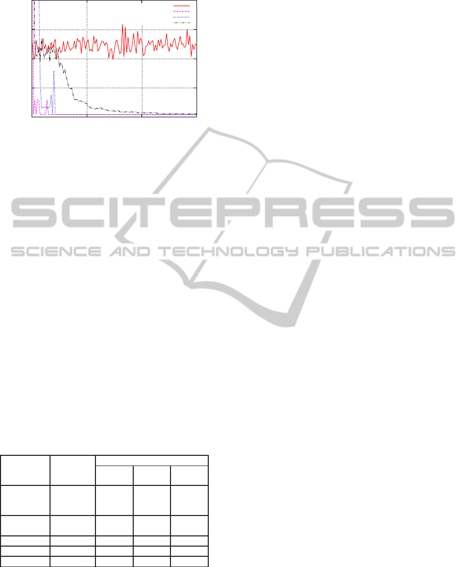
Figure 2: Average number of steps above first 60,000 tri-
als in the target task for R-MAX and TR-MAX using each
source task’s knowledge.
10 times for target task. In each execution, the agent
experiences 240,000 trials. Then, we calculated the
average steps that the agent consumes by reaching
the goal for each trail. Figure 2 shows the results
of the initial 60,000 trials because almost no change
occurred after 60,000 trials. TR-MAX converged at
about 10,000 to 20,000 trials, whereas R-MAX did
not converge within 60,000 trials. Moreover, we ob-
serve that the similarity of the source task to the tar-
get task affects the convergence speed. For instance,
among these three source tasks, Source task 1 in Fig-
ure 1(b) is the most similar to the target task in Fig-
ure 1(a), and “TR-MAX (Source task 1)” in Figure 2
converged the fastest among others. On the other
hand, “TR-MAX (Source task 3)” converged very
slowly, because Source task 3 in Figure 1(d) is not
similar to the target. In this sense, we verified that TR-
MAX could effectively utilize the prior knowledge.
Table 1: Sample complexities of R-MAX and TR-MAX us-
ing each source task’s knowledge. |Z
min|
is the minimum
size of the zero-transitioned state set, and |P
ε
| is the size of
the useful state-action pairs for the target task.
R-MAX
TR-MAX
Source
task 1
Source
task 2
Source
task 3
Sample
complexity
×10
7
4970 3.88 4.99 5.34
Ratio to
R-MAX
100% 0.078% 0.100% 0.107%
m 46742738 36550 46956 50243
|Z
min
| – 96 95 95
|P
ε
| – 376 304 196
Next, we compare the sample complexities of R-
MAX and TR-MAX in Table 1. As expected, the
sample complexities of TR-MAX are by far smaller
than the complexity of R-MAX, and they reflect the
similarities. We also note that the size |P
ε
| of the use-
ful state-action pairs P
ε
significantly depends on the
similarity, where the size |Z
min
| of the minimum zero-
transitioned sets does not.
5 CONCLUDING REMARKS
We proposed the TR-MAX algorithm that improved
the R-MAX algorithm by using prior knowledge for a
target task obtained from a source task. We proved
that the sample complexity of TR-MAX is indeed
smaller than that of R-MAX, and that TR-MAX is
PAC-MDP. In computationalexperiments, we verified
that TR-MAX could learn much more efficiently than
R-MAX.
In our future work, we are interested in capturing
“knowledge transfer in reinforcement learning” in an-
other way. In this position paper, we captured this as
a zero-transitioned state set and a useful state-action
pair set defined by the heuristic transition and heuris-
tic reward functions. In reality, however, these func-
tions cannot be obtained without knowing the true
transition and reward probabilities. In a real envi-
ronment, we never know the true probabilities, which
should be treated in future work.
REFERENCES
Brafman, R. I. and Tennenholtz, M. (2003). R-max - a gen-
eral polynomial time algorithm for near-optimal rein-
forcement learning. The Journal of Machine Learn-
ing, 3:213–231.
Kakade, S. M. (2003). On the Sample Complexity of Re-
inforceent Learning. PhD thesis, University College
London.
Konidaris, G. and Barto, A. (2006). Autonomous shaping:
Knowledge transfer in reinforcement learning. In Proc
of ICML, pages 489–496.
Kretchmar., R. M. (2002). Parallel reinforcement learning.
In Proc. of SCI, pages 114–118.
Mann, T. A. and Choe, Y. (2012). Directed exploration in
reinforcement learning with transferred knowledge. In
Proc. of EWRL, pages 59–76.
Miyazaki, K., Yamamura, M., and Kobayashi, S. (1997).
k-certainty exploration method: an action selector to
identify the environment in reinforcement learning.
Artificial intelligence, 91(1):155–171.
Rummery, G. A. and Niranjan, M. (1994). On-line Q-
learning using connectionist systems. Cambridge Uni-
versity.
Saito, J., Narisawa, K., and Shinohara, A. (2012). Predic-
tion for control delay on reinforcement learning. In
Proc. of ICAART, pages 579–586.
Schuitema, E., Busoniu, L., Babuska, R., and Jonker,
P. (2010). Control delay in reinforcement learning
ReducingSampleComplexityinReinforcementLearningby
TransferringTransitionandRewardProbabilities
637

for real-time dynamic systems: a memoryless ap-
proach. In Intelligent Robots and Systems (IROS),
2010 IEEE/RSJ International Conference on, pages
3226–3231. IEEE.
Strehl, A. L., Li, L., and Littman, M. L. (2009). Reinforce-
ment learning in finite mdps: Pac analysis. The Jour-
nal of Machine Learning Research, 10:2413–2444.
Strehl, A. L. and Littman, M. L. (2005). A theoretical anal-
ysis of model-based interval estimation. In Proc. of
ICML, pages 857–864.
Sutton, R. S. and Barto, A. G. (1998). Reinforcement learn-
ing. MIT Press.
Tan, M. (1993). Multi-agent reinforcement learning: In-
dependent vs. cooperative agents. In Proc. of ICML,
pages 330–337.
Taylor, M. E. and Stone, P. (2009). Transfer learning for re-
inforcement learning domains: A survey. The Journal
of Machine Learning Research, 10:1633–1685.
Taylor, M. E., Stone, P., and Liu, Y. (2007). Transfer
learning via inter-task mappings for temporal differ-
ence learning. Journal of Machine Learning Research,
8(1):2125–2167.
ICAART2014-InternationalConferenceonAgentsandArtificialIntelligence
638