A Heuristic Procedure with Local Branching for the Fixed Charge
Network Design Problem with User-optimal Flow
Pedro Henrique Gonz
´
alez
1,2
, Luidi Gelabert Simonetti
1
, Carlos Alberto de Jesus Martinhon
1
,
Philippe Yves Paul Michelon
2
and Edcarllos Santos
1
1
Institute of Computing, Fluminense Federal University, Niter
´
oi, Brazil
2
Laboratoire d’Informatique d’Avignon, Universit
´
e d’Avignon et des Pays de Vaucluse, Avignon, France
Keywords:
Network Design Problem, Heuristic, Local Branching, Bi-level Problem.
Abstract:
Due to the constant development of society, increasing quantities of commodities have to be transported in
large urban centers. Therefore, network design problems arise as tools to support decision-making, aiming
to meet the need of finding efficient ways to perform the transportation of each commodity from its origin
to its destination. This paper reviews a bi-level formulation, an one level formulation obtained by applying
the complementary slackness theorem, Bellman’s optimality conditions and Big-M linearizing technique. A
heuristic procedure is proposed, through combining a randomized constructive algorithm with a Relax-and-
Fix heuristic to generate an initial solution. After that a Local Branching technique is applied to improve
the constructed solution, so high quality solutions can be found. Besides that, our computational results are
compared with the results found in the literature, showing the efficiency of the proposed method.
1 INTRODUCTION
In the Fixed Charge Network Design Problem (FC-
NDP), a subset of edges are selected from a graph,
in such a way that a given set of commodities can
be transported from their origins to their destina-
tions. The main objective is to minimize the sum
of the fixed costs (due to selected edges) and vari-
able costs (depending on the flow of goods on the
edges). Fixed and variable costs can be represented
by linear functions and arcs are not capacitated. Be-
longing to a large class of network design problems
(Magnanti and Wong, 1984), the FCNDP has sev-
eral variations such as shortest path problem, min-
imum spanning tree problem, vehicle routing prob-
lem, traveling salesman problem and network Steiner
problem (Magnanti and Wong, 1984). For generic
network design problem, such as FCNDP, numer-
ous applications can be found (Boesch, 1976);(Boyce
and Janson, 1980);(Mandl, 1981), thus, mathemati-
cal formulations for the problem may also represent
several other problems, like problems of communi-
cation, transportation, sewage systems and resource
planning. It also appears in other contexts, such as
flexible production systems (Kimemia and Gershwin,
1978) and automated manufacturing systems (Graves
and Lamar, 1983). Finally, network design problems
arise in many vehicle fleet applications that do not in-
volve the construction of physical facilities, but rather
model decision problems such as sending a vehicle
through a road or not (Simpson, 1969); (Magnanti,
1981).
According to (Johnson et al., 1978);(Wong, 1978),
the simplest versions of network planning problems
are NP-Hard and even the task of finding feasible
solutions (for problems with budget constraint on
the fixed cost) is extremely complex (Wong, 1980).
Therefore, heuristics methods are presented as a good
alternative in the search for quality solutions.
This work is addressed for a specific variation of
FCNDP, called Fixed-Charge Uncapacited Network
Design Problem with User-optimal Flows (FCNDP-
UOF), which consists of adding multiple shortest
path problems to the original problem. The FCNDP-
UOF can be modeled as a bi-level discrete linear pro-
gramming problem which involves two distinct agents
acting simultaneously rather than sequentially when
making decisions. On the upper level, the leader (1
st
agent) selects a subset of edges to be opened in order
to minimize the sum of fixed and variable costs. In
response, on the lower level, the follower (2
nd
agent)
selects a set of shortest paths in the network, resulting
in the paths through which each commodity will be
sent. The effect of an agent on the other is indirect:
384
Henrique González P., Gelabert Simonetti L., Alberto de Jesus Martinhon C., Yves Paul Michelon P. and Santos E..
A Heuristic Procedure with Local Branching for the Fixed Charge Network Design Problem with User-optimal Flow.
DOI: 10.5220/0004885903840394
In Proceedings of the 16th International Conference on Enterprise Information Systems (ICEIS-2014), pages 384-394
ISBN: 978-989-758-027-7
Copyright
c
 2014 SCITEPRESS (Science and Technology Publications, Lda.)

the decision of the followers is affected by the net-
work designed on the upper level, while the leader’s
decision is affected by variable costs imposed by the
routes settled in the lower level.
Difficulties arise both in modeling and designing
efficient methods, mainly for the inclusion of short-
est path problem constraints in a mixed integer lin-
ear programming. Several variants could be seen on
(Billheimer and Gray, 1973); (Kara and Verter, 2004);
(Erkut et al., 2007); (Mauttone et al., 2008); (Erkut
and Gzara, 2008); (Amaldi et al., 2011); (Gonz
´
alez
et al., 2013) and have been treated as part of larger
problems in some applications on (Holmberg and
Yuan, 2004).
The FCNDP-UOF problem appears in the design
of a road network for hazardous materials transporta-
tion (Kara and Verter, 2004); (Erkut et al., 2007);
(Erkut and Gzara, 2008) and (Amaldi et al., 2011).
Particularly for this kind of problem, the govern-
ment defines a selection of road segments to be
opened/closed to the transportation of hazardous ma-
terials assuming that hazmat shipments in the result-
ing network will be done along shortest paths. In haz-
mat problems, roads selected to compose the network
have no costs, but the goverment wants to minimize
the population exposure in case of an incident during
a dangerous-goods transportation. This is a particu-
lar case of the FCNDP-UOF problem where the fixed
costs are equal zero.
It is interesting to specify the contributions of
each work cited above. (Billheimer and Gray, 1973)
present and formally define the FCNDP-UOF. (Kara
and Verter, 2004) and (Erkut et al., 2007) works focus
on exact methods, presenting a mathematical formu-
lation and several metrics for the hazardous materials
transportation problem. (Mauttone et al., 2008) not
only presented a different model, but also presented
a Tabu Search for the FCNDP-UOF. Both, (Erkut
and Gzara, 2008) and (Amaldi et al., 2011) presented
heuristic approaches to tackle the hazardous materi-
als transportation problem. At last, (Gonz
´
alez et al.,
2013), presented an extension of the model proposed
by Kara and Verter and also a GRASP.
This text is organized as follows. In Section 2, we
start by describing the problem followed by a bi-level
and an one-level formulation, presented by (Mauttone
et al., 2008). Then in Section 3 we present our so-
lution approach. Section 4 reports on our computa-
tional results. In Section 5 we compare our results
with heuristic results found in the literature. At last,
in Section 6 the conclusion and future works are pre-
sented.
2 GENERAL DESCRIPTION OF
FCNDP-UOF
In this section we formally introduce the problem and
present a bi-level and an one-level formulation for the
FCNDP-UOF proposed respectively by (Colson et al.,
2005) and (Mauttone et al., 2008) for the FCNDP-
UOF, which we address as MLF Model.
The problem is defined on a graph G = (V, E),
where V is a set of nodes that represent the facili-
ties and E is a set of of uncapacited and undirected
edges that represent the connection between installa-
tions. Furthermore, K is the set of commodities to
be transported over the network, which may represent
physical goods such as raw material for industry, haz-
ardous material or even people. For each commodity
k ∈ K, there is a flow to be delivered through a shortest
path between its source o(k) and its destination d(k).
Both formulations presented in this paper, work with
variants presenting commodities with multiple origins
and destinations, and for treating such a case, it is suf-
ficient to consider that for each pair (o(k), d(k)), there
is a new commodity resulting from the dissociation of
one into several commodities.
2.1 Mathematical Formulation
This subsection shows a small review of FCNDP-
UOF in order to exemplify the characteristics and fa-
cilitate its understanding.
Two kinds of variables can be noticed for FCNDP-
UOF model, one for the construction of the network
and another related to representing the flow. Let y
i j
be a binary variable, we have that y
i j
= 1if the edge
(i, j) is chosen as part of the network and y
i j
= 0 oth-
erwise. In this case, x
k
i j
denotes the commodity k flow
through the arc (i, j). Although the edges have no di-
rection, they may be referred to as arcs, because each
commodity flow is directed. Treating y = (y
i j
) and
x = (x
k
i j
), respectively, as vectors of adding edge and
flow variables, a mixed integer programming formu-
lation can be elaborated.
2.1.1 List of Symbols
V Set of Nodes.
E Set of admissible bi-directed Edges.
K Set of Commodities.
δ
+
i
Set of all arcs leaving node i.
δ
−
i
Set of all arcs arriving at node i.
c
e
Length of edge e.
o(k) Origin node for commodity k.
d(k) Destination node for commodity k.
AHeuristicProcedurewithLocalBranchingfortheFixedChargeNetworkDesignProblemwithUser-optimalFlow
385

g
k
i j
Variable cost of transporting commodity
k through the edge (i, j) ∈ E.
f
i j
Fixed cost of opening the edge (i, j) ∈ E.
y
i j
Indicates if edge (i, j) belongs in the solution.
x
k
i j
Indicates if commodity k passes through
the arc (i, j).
2.1.2 Bi-level Formulation
In FCNDP-UOF, different from the basic FCNDP,
each commodity k ∈ K has to be transported through
a shortest path between its origin o(k) and its destina-
tion d(k), thus forcing the adding of new constraints
to the general problem. Besides selecting a subset of
E whose sum of fixed and variable costs is minimal
(leading problem), in this variation, each commod-
ity k ∈ K must be transported through the shortest
path between o(k) and d(k) (follower problem). The
FCNDP-UOF belongs to the class of NP-Hard prob-
lems and can be modeled as a bi-level discrete integer
programming problem (Colson et al., 2005), as fol-
lows:
min
∑
(i, j)∈E
f
i j
y
i j
+
∑
k∈K
∑
(i, j)∈E
g
k
i j
x
k
i j
s.t. y
i j
∈ {0, 1}, ∀e = (i, j) ∈ E,
(1)
where x
k
i j
is a solution of the problem:
min
∑
k∈K
∑
(i, j)∈E
c
i j
x
k
i j
s.t.
∑
(i, j)∈δ
+
(i)
x
k
i j
−
∑
(i, j)∈δ
−
(i)
x
k
i j
= b
k
i
, ∀i, j ∈ V, ∀k ∈ K,
x
k
i j
+ x
k
ji
≤ y
e
, ∀e = (i, j) ∈ E, ∀k ∈ K,
x
k
i j
≥ 0, ∀e = (i, j) ∈ E, ∀k ∈ K.
(2)
(3)
(4)
where:
b
k
i
=
(
−1 if i = d(k),
1 if i = o(k),
0 otherwise.
According to constraints (1)-(4), we can notice
that the set of constraints (1) ensures that y
e
assume
only binary values. In (2), we have flow constraints.
Constraints (3) do not allow flow into arcs whose cor-
responding edges are closed. Finally, (4) imposes the
non-negativity restriction of the variables x
k
i j
. An in-
teresting remark is that solving the follower problem
is equivalent to solving |K| shortest path problems in-
dependently.
2.1.3 One-level Formulation
The FCNDP-UOF can be formulated as an one-level
integer programming problem replacing the objective
function and the constraints defined by (2), (3) and
(4) of the follower problem for its optimality condi-
tions (Mauttone et al., 2008). This replacing can be
done applying the fundamental theorem of duality and
the complementary slackness theorem (Bazaraa et al.,
2004). However, optimality conditions for the prob-
lem in the lower level are, in fact, the optimality con-
ditions of the shortest path problem and they could be
expressed in a more compact and efficient way if we
consider the Bellman’s optimality conditions for the
shortest path problem (Ahuja et al., 1993) and using a
simple lifting process (Luigi De Giovanni, 2004).
A disadvantage of this new formulation is the loss
of linearity for the model. To bypass this problem
we use a Big-M linearization. After these, we can
write the model as an one-level mixed integer linear
programming problem, as follows:
min
∑
(i, j)∈E
f
i j
y
i j
+
∑
k∈K
∑
(i, j)∈E
g
k
i j
x
k
i j
s.t.
∑
(i, j)∈δ
+
(i)
x
k
i j
−
∑
(i, j)∈δ
−
(i)
x
k
i j
= b
k
i
, ∀i, j ∈ V,∀k ∈ K,
x
k
i j
+ x
k
ji
≤ y
i j
, ∀e = (i, j) ∈ E, ∀k ∈ K,
π
k
i
− π
k
j
≤ M − y
e
(M − c
e
) − 2c
e
x
k
ji
, ∀e = (i, j) ∈ E, k ∈ K,
π
k
i
≥ 0, ∀i ∈ V, ∀k ∈ K,
π
k
i
= 0, ∀i = d(k), ∀k ∈ K,
π
k
i
∈ R, ∀i ∈ V, ∀k ∈ K,
x
k
i j
∈ {0, 1}, ∀(i, j) ∈ E, ∀k ∈ K,
y
i j
∈ {0, 1}, ∀(i, j) ∈ E.
(5)
(6)
(7)
(8)
(9)
(10)
(11)
(12)
where:
b
k
i
=





−1 if i = d(k),
1 if i = o(k),
0 otherwise.
The variables π
k
i
, k ∈ K, i ∈ V, are the shortest
distance between vertex i and vertex d(k). Then we
define that π
k
d(k)
will always be equal zero. Assum-
ing y and x binary and assuming that the inequalities
(7) are satisfied, it is easy to see that constraints (8)
are equivalent to Bellman’s optimality conditions for
a |K| set of pairs (o(k), d(k)).
3 SOLUTION APPROACH
This section focuses on the Partial Decoupling
Heuristic, the Relax and Fix Heuristic and the Local
Branching techniques. After explaining those compo-
nents, we introduce a heuristic procedure combining
all three methods.
ICEIS2014-16thInternationalConferenceonEnterpriseInformationSystems
386

3.1 Partial Decoupling Heuristic
The main idea of total decoupling heuristic for the
FCNDP-UOF is dissociating the problem of building
a network from the shortest path problem. This dis-
integration, as discussed in (Erkut and Gzara, 2008),
can provide worst results than when addressing both
problems simultaneously. To work around this situa-
tion, the algorithm proposes what we call partial de-
coupling, where certain aspects of the follower prob-
lem are considered when trying to build a solution to
the leading problem. So in order to build the network
the following cost is used: ( f
e
×(1− y
e
))+(α ×g
k
0
i j
+
(1 − α) × c
e
), which means that we consider whether
the is edge open or not, plus a linear combination of
the variable cost and the length of the edge. The α
works as a mediator of the importance of the g
k
0
i j
and
c
e
values. In the beginning of the iterations α priori-
tizes the variable cost (g
k
0
i j
), while in the end it priori-
tizes the edge length (c
e
).. After building the network,
a shortest path algorithm is applied to take every prod-
uct from its origin o(k) to its destination d(k). In this
situation, is important to note that g
k
i j
= q
k
β
i j
, where
q
k
represents the amount of commodity k and β
i j
rep-
resents the shipping cost through the edge e = (i, j).
Initially presented in (Gonz
´
alez et al., 2013), the pro-
posed algorithm is a small variation of the original
Partial Decoupling Heuristic. The procedure is fur-
ther explained on Algorithm 1.
To solve the shortest path problem, the partial de-
coupling heuristic applies the Dijkstra algorithm. At
first, the procedure DijkstraLeader solves the prob-
lem of network construction, then, the shortest path
problem is solved for each commodity k ∈ K using
the DijkstraFollower procedure, so that in the end of
these procedures, all commodities have been trans-
ported from its origin to its destination. The proce-
dure costs for DijkstraLeader and DijkstraFollower
are respectively DLCost and DSCost. The notation
s ←< y, x > means that the solution s is storing the
values of the variables y and x that were just defined
by DijkstraLeader and DijkstraFollower. Since the
procedure DijskstraFollower can open edges that do
not have flow, we used the function CloseEdge to
close theses edges. The Random function returns a
random element from the set passed as a parameter.
In order to choose the insertion order of |K| com-
modities, the procedure uses a candidate list consist-
ing of a subset of commodities not yet routed, whose
amount is greater than or equal to γ times the largest
amount of the commodity not routed. The function
Rearm(K) adds all commodities to set K and makes
all variables return to their initial state.
Algorithm 1: Partial Decoupling Heuristic.
Input: γ
Data: MinCost ← ∞, α ← 1, y ← 0, x ← 0;
begin
¯
K ← K;
for numIterDP in 1 . . . MaxIterDP do
while K 6=
/
0 do
K ← CandidateList(K, γ);
k
0
← Random(K);
for each e = (i, j) ∈ E do
DLCost(e, k
0
) ← ( f
e
× (1 − y
e
)) +
(α × g
k
0
i j
+ (1 − α) × c
e
);
y ← Di jkstraLeader(DLCost, k
0
);
K ← K\{k
0
};
for each e = (i, j) ∈ E do
DSCost(e) ← c
e
;
for k ∈
¯
K do
x ← Di jkstraFollower(DSCost, k);
s ←< y, x >;
CloseEdge(s);
if Cost(s) < MinCost then
s
best
← s;
MinCost ← Cost(s
best
);
α ← α −
1
MaxIterDP
;
Rearm(K);
return s
best
3.2 Relax and Fix Heuristic
Given a mixed integer programming formulation:







min c
1
z
1
+ c
2
z
2
;
s.t. A
1
z
1
+ A
2
z
2
= b;
z
1
∈ Z
n
+
, z
2
∈ Z
n
+
;
(13)
(14)
without loss of generality, let’s suppose that the vari-
ables z
1
j
for j ∈ N
1
are more important than the vari-
ables z
2
j
for j ∈ N
2
, with n
i
= |N
i
| for i = 1,2.
The idea of the Relax and Fix, consists in solving
two (or more) easier LPs or MIPs. The first one allows
us to fix (i.e. z
i
j
= w, w ∈ Z
n
i
+
) or limit the range of
more important variables, while the second allows us
to choose good values for other variables z
2
.
In order to do so, first it is necessary to solve a
relaxation like:







min c
1
z
1
+ c
2
z
2
;
s.t. A
1
z
1
+ A
2
z
2
= b;
z
1
∈ Z
n
1
+
, z
2
∈ R
n
2
+
;
(15)
(16)
in which the integrality of z
2
variables is dropped. Let
(¯z
1
, ¯z
2
) be the corresponding solution. Secondly fix
the important variables, according to criterias based
AHeuristicProcedurewithLocalBranchingfortheFixedChargeNetworkDesignProblemwithUser-optimalFlow
387

on the problem peculiarity, and solve the new prob-
lem. After that, (¯z
1
, ¯z
2
) becomes the corresponding
solution if the solution of the relaxed model is feasi-
ble. At last, the algorithm returns z
H
= (¯z
1
,
¯
¯z
2
).
In terms of algorithm, the Relax and Fix procedure
can be seen as:
Algorithm 2: Relax and Fix Heuristic.
Input: n
1
, n
2
, N
1
, N
2
Data: MinCost ← ∞
begin
for i = 1 . . . 2 do
for j ∈ N
2
do
z
j
i
∈ {0, 1};
s ← SolveLR(N
1
, N
2
);
for j ∈ N
1
do
if z
j
i
= w then
z
j
i
= w;
if Cost(s) < MinCost and
Feas(s) = T RUE then
s
best
← s ;
MinCost ← Cost(s
best
) ;
return s
best
The function SolveLR(N
1
, N
2
) solves the linear
relaxation of the Generalized Model for the sets N
1
and N
2
. Since z
j
i
are decision variables in the integer
programming model, the symbol ∈ is used to express
the idea of limiting the variation of the variable value
during the branch-and-bound algorithm, which also
means fixing it as the real number w. The function
Feas(s) returns true if the solution s passed as param-
eter is a feasible solution to the problem and returns
false otherwise.
3.3 DPRF
In order to adapt the Relax and Fix for the FCNDP-
UOF, we separate the set of variables x
k
i j
, (i, j) ∈ E,
k ∈ K, in |K| disjoint sets, where |K| is the number of
commodities on the model, so that the heuristic per-
forms |K| iterations. At each iteration k, the variables
x
k
i j
∈ Q
k
are defined as binary. After solving the re-
laxed model, if it returns a feasible solution, we fix
the variables y
e
, that are both zero and attend to the
reduced cost criterion for variable fixing, as zero.
The function SolveLR(V, E, K, MinCost) solves the
linear relaxation of the MLF Model for the sets V ,
E and K, taking into consideration the primal bound
MinCost. The RCV F(y
e
) function returns TRUE if
the Linear Relaxation cost plus the Reduced Cost of
y
e
is lower than the current Relax and Fix solution.
Since y
e
and x
k
e
are decision variables in the integer
programming model, the symbol ∈ is used to express
the idea of limiting the variation of the variable value
during the branch-and-bound algorithm, even if the
variable is set to a single value (i.e y
e
∈ {0}). The
function Feas(s) returns true if the solution s passed
as parameter is a feasible solution to the problem and
returns false otherwise.
Algorithm 3: DPRF.
Input: γ
Data: MinCost ← ∞
begin
s ← PartialDecoupling(γ);
MinCost ← Cost(s) ;
¯
K ← K;
while
¯
K 6=
/
0 do
k ← CandidateList(
¯
K, γ);
for e ∈ E do
x
k
e
∈ {0, 1};
s ← SolveLR(V, E, K, MinCost);
for e ∈ E do
if y
e
= 0 and RCV F(y
e
) = T RUE
then
y
e
∈ {0};
if Cost(s) < MinCost and
Feas(s) = T RUE then
s
best
← s ;
MinCost ← Cost(s
best
) ;
return s
best
In order to choose the order of x
k
i j
variables to become
binary, the procedure uses a candidate list. In order to
choose a commodity, a candidate list consisting of the
commodities whose amount is greater than or equal
to γ times the largest amount of the commodity whose
variables are not set as binary.
It is important to remark that the DPRF proce-
dure presented here is a variation of the DPRF proce-
dure presented in the paper ”An Improved Relax-and-
Fix Algorithm for the Fixed Charge Network Design
Problem with User-optimal Flow”, which has been
sent to ICORES 2014 on September, 2013.
3.4 Local Branching
Introduced by (Fischetti and Lodi, 2003), the Local
Branching (LB) technique could be used as a way of
improving a given feasible solution.
The LB makes use of a MIP solver to explore the
solution subspaces effectively. The procedure can be
seen as local search, but the neighborhoods are ob-
tained through the introduction of linear inequalities
ICEIS2014-16thInternationalConferenceonEnterpriseInformationSystems
388

in the MIP model, called local branching cuts. More
specifically, the LB searches for a local optimum by
restricting the number of variables, from the feasible
solution, whose values can be changed.
Formally speaking, consider a feasible solution
of the FCNDP-UOP, s =< ¯y, ¯x >∈ P, where P is a
polyhedron. The general idea would be adding the
LB constraint
∑
e∈E| ¯y
e
=0
y
e
+
∑
e∈E| ¯y
e
=1
(1 − y
e
) ≤ ∆, (17)
where ∆ is a given positive integer parameter, indicat-
ing the number of variables y
e
, e ∈ E, that are allowed
to flip from one to zero and vice versa. The strategy
used here consists on applying the LB constraint only
on y variables, leaving x
k
i j
variables free of LB con-
straints.
3.5 Heuristic for FCNDP-UOF
The proposed heuristic has two main components,
the DPRF and the Local Branching. The methods
are applied in a straightforward way. First we ran
the DPRF to get a feasible solution. Secondly we
try to improve the quality of the previously found
solution through applying the Local Branching. The
algorithm is described in Algorithm 4.
Algorithm 4: DPRFLB.
Input: γ, ∆
begin
s ← DPRF(γ);
s
best
← s;
¯s ← LB(s
best
, ∆);
if Cost( ¯s) ≤ Cost(s
best
) then
s
best
← ¯s;
return s
best
In DPRFLB, the initial solution is generated by
the DPRF. Then, the function LB performs a Local
Branching Technique. The function Primal-Bound
updates the solver primal bound, in order to avoid ex-
ploring uninteresting nodes of the branch-and-bound
tree.
4 COMPUTATIONAL RESULTS
In this section we present computational results for
the method presented in the previous section.
The algorithm was coded in Xpress Mosel using
FICO Xpress Optimization Suite, on an Intel (R) Core
TM i7 - 4700MQ CPU @ 2.4 GHz computer with
16GB of RAM. Computing times are reported in sec-
onds. In order to test the performance of the presented
heuristic, we used networks data obtained through
private communication with Mauttone, Labbe and
Figueiredo.
In order to calibrate the algorithms the following
γ and ∆ values were tested: γ = {0.75, 0.85, 0.90} and
∆ = {d
|E|
4
e, d
|E|
3
e, d
|E|
2
e}. After the tests the following
values were selected: γ = 0.85 and ∆ = d
|E|
2
e.
The data used are grouped according to the num-
ber of nodes in the graph (10, 20, 30),followed by the
graph density (0.3, 0.5, 0.8) and finally the amount
of different commodities to be transported. For the
presented tables, we report the optimum value found
by exact model (Opt), the best solution (Best Sol) and
best time (Best Time) reached by selected approach,
and the gap value between exact and heuristic (GAP).
We also reported the average values for time (Avg
Time) and for solutions (Avg Sol). Finally, reported
standard deviation values for time(Dev Time) and so-
lution(Dev Sol)
In both tables the results in bold represent the best
solution found, while the underlined ones represent
that the optimum has been found.
In Table 1, we present the results reached for
the instances generated by (Mauttone et al., 2008).
For these five instances, two heuristics were com-
pared: the GRASP heuristic of (Gonz
´
alez et al., 2013)
(whose results were superior to those obtained by the
tabu search presented by (Mauttone et al., 2008) and
the DPRFLB algorithm). When observing the gap
value, the table shows that the GRASP heuristic ob-
tained best solutions in general, however the com-
putational time is very high in comparison with the
DPRFLB heuristic. Moreover, the standard deviation
obtained by GRASP presented high values suggest-
ing the algorithm has a irregular behavior and for the
DPRFLB algorithm all standard deviation values for
solutions were 0.
In Table 2 were used another 45 instances gener-
ated by Mautonne, Labb and Figueiredo, whose re-
sults were not published by them. For this group of
instances, the computational results suggest the effi-
ciency of DPRFLB heuristic. On average, the time
spent by DPRFLB was 8.35 times faster than the time
spent by GRASP. Also, DPRFLB found 40 optimal
solutions, while GRASP found only 7 optimal solu-
tions. Besides that, the DPRFLB also improved or
equaled GRASP results for 44 (37 improvements) out
of 45 instances.
In tables 1 and 2 the result states, at least for the
instances tested, the order of the commodities set by
the candidate list in the DPRFLB does not affect the
AHeuristicProcedurewithLocalBranchingfortheFixedChargeNetworkDesignProblemwithUser-optimalFlow
389

Table 1: Computational results for GRASP and DPRFLB approach for |V | = 30.
GRASP DPRFLB
Avg Sol Avg Time Dev Sol Dev Time Best Sol Best Time GAP Avg Sol Avg Time Dev Time Best Sol Best Time GAP
30-0.8-30-001 4871 332.14 0 9.22 4871 330.908 0.008 4830 33.55 0.06 4830 32.91 0.000
30-0.8-30-002 7122.2 328.29 182.39 4.11 6989 325.357 0 7322 81.71 0.09 7322 80.437 0.048
30-0.8-30-003 8124 337.19 16.43 33.63 8112 321.838 0.047 8112 158.98 0.19 8112 155.709 0.047
30-0.8-30-004 8384 318.06 0 26.09 8384 338.249 0 8755 176.94 0.04 8755 174.63 0.044
30-0.8-30-005 7442.8 321.43 33.09 17.89 7428 344.367 0 7428 135.51 0.04 7428 134,18 0,000
Avg 327.42 0.011 117.33 0.028
Table 2: Computational results for GRASP and DPRFLB approach for |V | = 20.
GRASP DPRFLB
Avg Sol Avg Time Dev Sol Dev Time Best Sol Best Time GAP Avg Sol Avg Time Dev Time Best Sol Best Time GAP
20-0.3-10-001 6513.58 15.65 136.48 0.34 6411 15.50 0.07 5978 0.62 0.00 5978 0.61 0.00
20-0.3-10-002 10813.30 16.57 185.69 0.58 10664 16.38 0.02 10469 3.24 0.01 10469 3.218 0.00
20-0.3-10-003 7286.40 15.99 132.14 0.34 7200 15.67 0.03 7020 4.07 0.02 7020 4.027 0.00
20-0.3-10-004 5754.74 15.84 116.73 0.33 5598 15.71 0.02 5484 4.06 0.02 5484 4.024 0.00
20-0.3-10-005 8322.00 16.04 0.00 0.40 8322 16.01 0.05 7932 1.41 0.01 7932 1.4 0.00
20-0.3-20-001 9488.00 32.10 0.00 1.36 9488 31.84 0.00 9488 0.78 0.00 9488 0.778 0.00
20-0.3-20-002 11699.86 31.64 201.31 0.91 11607 30.94 0.01 11521 5.02 0.02 11521 4.978 0.00
20-0.3-20-003 8670.82 32.57 222.90 0.72 8568 32.44 0.04 8270 1.32 0.01 8270 1.311 0.00
20-0.3-20-004 12320.58 31.94 300.06 1.07 11985 31.62 0.01 11990 5.46 0.02 11990 5.416 0.01
20-0.3-20-005 10379.38 32.12 178.59 0.46 10297 31.93 0.07 9656 1.29 0.01 9656 1.281 0.00
20-0.3-30-001 13244.00 49.28 0.00 0.76 13244 48.69 0.06 12510 1.64 0.01 12510 1.629 0.00
20-0.3-30-002 14854.90 49.81 364.81 1.76 14737 49.41 0.04 14216 1.68 0.01 14216 1.666 0.00
20-0.3-30-003 14687.52 48.18 577.28 1.41 14629 47.79 0.09 13393 10.10 0.04 13393 10.009 0.00
20-0.3-30-004 15420.97 48.62 327.77 0.63 15329 48.32 0.06 14452 2.07 0.01 14452 2.055 0.00
20-0.3-30-005 12599.00 51.32 0.00 1.08 12599 51.02 0.10 11419 1.40 0.01 11419 1.393 0.00
20-0.5-10-001 4784.00 21.56 0.00 0.83 4784 21.43 0.00 4784 1.18 0.00 4784 1.174 0.00
20-0.5-10-002 7689.00 21.86 0.00 0.57 7689 21.73 0.00 7689 1.49 0.01 7689 1.478 0.00
20-0.5-10-003 6184.00 22.68 0.00 0.47 6184 22.45 0.00 6184 0.65 0.00 6184 0.647 0.00
20-0.5-10-004 5532.91 22.41 95.20 0.29 5489 22.19 0.06 5189 1.18 0.01 5189 1.165 0.00
20-0.5-10-005 6233.72 22.78 80.47 0.59 6172 22.74 0.02 6051 6.90 0.03 6051 6.842 0.00
20-0.5-20-001 9964.00 46.50 0.00 0.95 9964 45.85 0.13 8816 2.88 0.01 8816 2.858 0.00
20-0.5-20-002 8721.34 47.45 150.45 1.83 8584 46.89 0.00 8584 1.80 0.01 8584 1.783 0.00
20-0.5-20-003 8354.83 45.72 214.84 0.92 8305 44.65 0.10 7560 8.73 0.04 7560 8.646 0.00
20-0.5-20-004 7750.74 45.28 100.06 0.84 7674 44.92 0.01 7634 1.39 0.01 7634 1.383 0.00
20-0.5-20-005 8636.00 44.86 0.00 1.12 8636 44.77 0.04 8270 9.63 0.04 8270 9.553 0.00
20-0.5-30-001 12600.00 67.99 0.00 2.34 12600 67.99 0.24 10156 2.12 0.01 10156 2.106 0.00
20-0.5-30-002 12932.00 68.66 0.00 1.91 12932 68.66 0.13 11403 9.73 0.04 11403 9.644 0.00
20-0.5-30-003 13021.40 73.29 334.74 1.35 12867 71.57 0.11 11600 14.94 0.06 11600 14.815 0.00
20-0.5-30-004 12333.56 70.88 317.15 1.32 12260 68.82 0.04 11794 8.78 0.04 11794 8.705 0.00
20-0.5-30-005 10989.00 69.47 0.00 1.82 10989 69.33 0.15 9559 4.84 0.02 9559 4.795 0.00
20-0.8-10-001 4120.80 34.32 105.35 0.90 4040 34.32 0.02 3947 0.38 0.00 3947 0.379 0.00
20-0.8-10-002 3915.00 34.51 0.00 1.13 3915 34.02 0.05 3743 5.32 0.02 3743 5.275 0.00
20-0.8-10-003 3480.24 34.81 74.75 0.58 3412 34.39 0.00 3412 0.37 0.00 3412 0.366 0.00
20-0.8-10-004 4209.00 35.27 0.00 0.80 4209 34.99 0.03 4086 6.69 0.03 4086 6.633 0.00
20-0.8-10-005 4542.98 35.64 97.51 0.77 4498 35.28 0.00 4498 2.22 0.01 4498 2.196 0.00
20-0.8-20-001 6909.00 70.88 0.00 1.73 6909 69.22 0.19 5796 3.38 0.01 5796 3.349 0.00
20-0.8-20-002 7635.54 71.48 187.03 1.02 7590 70.34 0.08 7321 30.01 0.13 7321 29.744 0.04
20-0.8-20-003 6251.89 69.00 89.48 1.84 5422 68.18 0.18 4596 8.01 0.04 4596 7.937 0.00
20-0.8-20-004 5250.00 70.26 69.01 2.45 5187 69.98 0.08 4851 2.73 0.01 4851 2.71 0.00
20-0.8-20-005 6855.53 72.13 86.23 1.93 6267 71.42 0.03 6086 14.91 0.06 6086 14.781 0.00
20-0.8-30-001 9425.00 105.01 0.00 2.17 9425 101.23 0.21 7769 8.07 0.04 7769 8 0.00
20-0.8-30-002 8735.33 110.77 126.42 1.98 8666 109.89 0.13 7681 11.87 0.05 7681 11.78 0.00
20-0.8-30-003 5947.89 107.30 201.43 2.67 5889 106.24 0.14 5595 7.66 0.03 5595 7.596 0.09
20-0.8-30-004 8768.08 104.77 177.53 3.74 8630 104.56 0.20 7387 29.02 0.11 7387 28.799 0.03
20-0.8-30-005 8175.16 108.08 127.82 1.46 7942 108.08 0.08 7374 16.98 0.07 7374 16.83 0.00
Avg 2 49,32 0,07 5,91 0,003
ICEIS2014-16thInternationalConferenceonEnterpriseInformationSystems
390

quality of the solution, but do affect the computational
time.
4.1 Statistical Analysis
In order to verify whether or not the differences
of mean values obtained by the evaluated strategies
shown in Tables 1 and 2 are statistically significant,
we employed the Wilcoxon-Mann-Whitney test tech-
nique (Hettmansperger and McKean, 1998). This test
could be applied to compare algorithms with some
random features and identify if the difference of per-
formance between them is due to randomness.
According to (Hettmansperger and McKean,
1998), this statistical test is used when two indepen-
dent samples are compared and whenever it is nec-
essary to have a statistical test to reject the null hy-
pothesis, with a significance θ level (i.e., it is possible
to reject the null hypothesis with the probability of
(1 −θ×100%)). For the sake of this analysis we con-
sidered θ = 0.01. The hypotheses considered in this
test are:
• Null Hypothesis (H0): there are no significant dif-
ferences between the solutions found by DPRFLB
and the original method;
• Alternative Hypothesis (H1): there are significant
differences (bilateral alternative) between the so-
lutions found by DPRFLB and the GRASP.
Table 3 presents the number of better average so-
lutions found by each strategy, for each group of the
same size instances. The number of cases where the
Null Hypothesis was rejected is also shown between
parentheses.
Table 3: Statistical Analysis of GRASP and DPRFLB.
Algorithms
Instance Group
20 30
GRASP 0(0) 2(2)
DPRFLB 41(37) 3(1)
When comparing GRASP with DPRFLB, we no-
tice that almost all differences of performance (80%
of the tests) are statistically significant. We can also
observe that the DPRFLB obtained 88% of the best
results. These results indicate the superiority of the
proposed strategy.
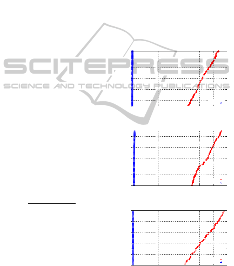
4.2 Complementary Analysis
Thanks to time-to-target plots (TTT-plots) ((Aiex and
Ribeiro, 2006)), we have another tool to analyze
the behavior of algorithms with random components.
These plots show the cumulative probability of an al-
gorithm reaching a prefixed target solution in the in-
dicated running time. In TTT-plots experiment, we
sorted out the execution times required for each algo-
rithm to reach a solution at least as good as a prede-
fined target solution. After that, the i-th sorted run-
ning time, t
i
, is associated with a probability p
i
=
i−0.5
100
and the points z
i
= (t
i
; p
i
) are plotted.
For this experiments we tested 10 of our largest
instances with a medium target. Firstly we analyze
the instances with 20 nodes, followed by the analyses
of instances with 30 nodes.
After analyzing the behavior of the methods for
the biggest instances of 20 nodes, through analysis of
the TTTPlot graphics 1 to 5, we conclude that the pro-
0
0.1
0.2
0.3
0.4
0.5
0.6
0.7
0.8
0.9
1
0 20 40 60 80 100 120 140
Cumulative Probability
Time to Target Solution (s)
GRASP
DPRFLB
Figure 1: TTTPlot - Medium Target - 20-0800000-30-001.
0
0.1
0.2
0.3
0.4
0.5
0.6
0.7
0.8
0.9
1
0 20 40 60 80 100 120 140
Cumulative Probability
Time to Target Solution (s)
GRASP
DPRFLB
Figure 2: TTTPlot - Medium Target - 20-0800000-30-002.
0
0.1
0.2
0.3
0.4
0.5
0.6
0.7
0.8
0.9
1
0 20 40 60 80 100 120 140
Cumulative Probability
Time to Target Solution (s)
GRASP
DPRFLB
Figure 3: TTTPlot - Medium Target - 20-0800000-30-003.
AHeuristicProcedurewithLocalBranchingfortheFixedChargeNetworkDesignProblemwithUser-optimalFlow
391

0
0.1
0.2
0.3
0.4
0.5
0.6
0.7
0.8
0.9
1
0 20 40 60 80 100 120 140 160
Cumulative Probability
Time to Target Solution (s)
GRASP
DPRFLB
Figure 4: TTTPlot - Medium Target - 20-0800000-30-004.
0
0.1
0.2
0.3
0.4
0.5
0.6
0.7
0.8
0.9
1
0 20 40 60 80 100 120 140
Cumulative Probability
Time to Target Solution (s)
GRASP
DPRFLB
Figure 5: TTTPlot - Medium Target - 20-0800000-30-005.
0
0.1
0.2
0.3
0.4
0.5
0.6
0.7
0.8
0.9
1
0 50 100 150 200 250 300 350
Cumulative Probability
Time to Target Solution (s)
GRASP
DPRFLB
Figure 6: TTTPlot - Medium Target - 30-0800000-30-001.
posed strategy outperforms the GRASP The cumula-
tive probability for DPRFLB to find the target in less
then 50 seconds is 100 %, while for GRASP is 0 %.
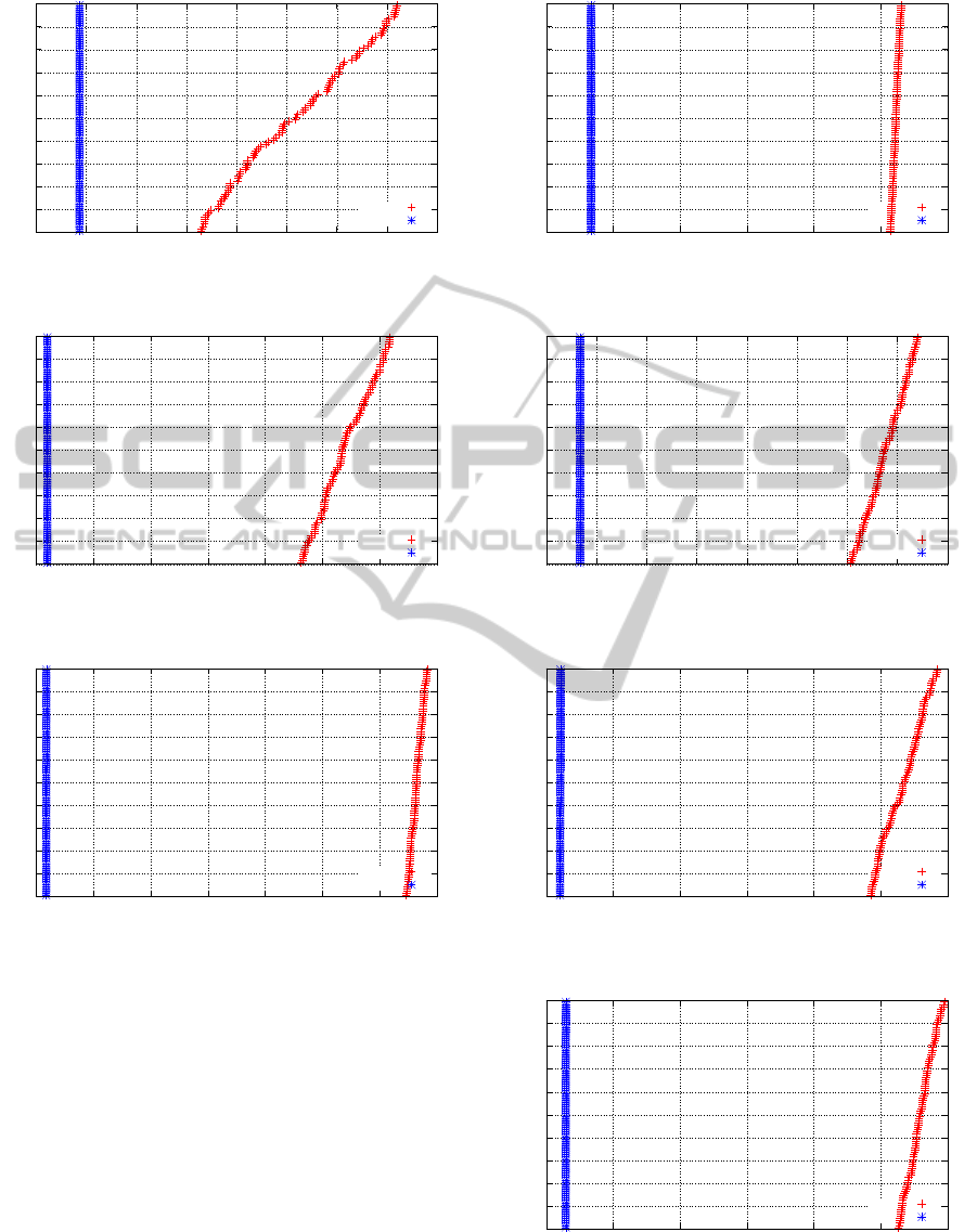
After analyzing the behavior of the methods for
the biggest instances of 30 nodes, through analysis of
the TTTPlot graphics 6 to 10, we conclude that even
though GRASP outperformed the DPRFLB in the sta-
tistical analysis, DPRFLB finds medium targets faster
than GRASP.
Once again, the cumulative probability for
DPRFLB to find the target in less then 50 seconds is
100 %, while for GRASP is 0 %.
0
0.1
0.2
0.3
0.4
0.5
0.6
0.7
0.8
0.9
1
0 50 100 150 200 250 300
Cumulative Probability
Time to Target Solution (s)
GRASP
DPRFLB
Figure 7: TTTPlot - Medium Target - 30-0800000-30-001.
0
0.1
0.2
0.3
0.4
0.5
0.6
0.7
0.8
0.9
1
0 50 100 150 200 250 300 350 400
Cumulative Probability
Time to Target Solution (s)
GRASP
DPRFLB
Figure 8: TTTPlot - Medium Target - 30-0800000-30-003.
0
0.1
0.2
0.3
0.4
0.5
0.6
0.7
0.8
0.9
1
50 100 150 200 250 300 350
Cumulative Probability
Time to Target Solution (s)
GRASP
DPRFLB
Figure 9: TTTPlot - Medium Target - 30-0800000-30-004.
0
0.1
0.2
0.3
0.4
0.5
0.6
0.7
0.8
0.9
1
0 50 100 150 200 250 300
Cumulative Probability
Time to Target Solution (s)
GRASP
DPRFLB
Figure 10: TTTPlot - Medium Target - 30-0800000-30-005.
ICEIS2014-16thInternationalConferenceonEnterpriseInformationSystems
392

5 CONCLUSIONS
We proposed a new algorithm for a variant of the
fixed-charge uncapacitated network design problem
where multiple shortest path problems are added to
the original problem. In the first phase of the algo-
rithm, the DPRF is used to build a initial solution. In
the second phase, a Local Branching technique is ap-
plied to reduce the solution cost.
The proposed approach was tested on a set of in-
stances grouped by graph density, number of nodes
and commodities. Our results have shown the effi-
ciency of DPRFLB in comparison with the GRASP
presented by (Gonz
´
alez et al., 2013), once the pro-
posed algorithm presented best average time for all
instances, often reaching optimum solutions (42 out
of 50). In a few cases, GRASP reached best solution
values, however not only the computational time was
elevated when compared with DPRFLB, but also just
two results were statistically significant.
As future work, we intend to work on the math-
ematical formulation and implement a ILS (Loureno
and S., 2010) metaheuristic taking into consideration
the components presented here.
ACKNOWLEDGEMENTS
This work was supported by CAPES (Process
Number: BEX 9877/13-4) and by Laboratoire
d’Informatique d’Avignon, Universit d’Avignon et
des Pays de Vaucluse, Avignon, France.
REFERENCES
Ahuja, R. K., Magnanti, T. L., and Orlin, J. B. (1993).
Network flows: theory, algorithms, and applications.
Prentice-Hall, Inc., Upper Saddle River, NJ, USA.
Aiex, R. M., R. M. G. C. and Ribeiro, C. C. (2006). Ttt
plots: A perl program to create time-to-target plots.
Optimization Letters.
Amaldi, E., Bruglieri, M., and Fortz, B. (2011). On the haz-
mat transport network design problem. In Proceed-
ings of the 5th international conference on Network
optimization, INOC’11, pages 327–338, Berlin, Hei-
delberg. Springer-Verlag.
Bazaraa, M. S., Jarvis, J. J., and Sherali, H. D. (2004).
Linear Programming and Network Flows. Wiley-
Interscience.
Billheimer, J. W. and Gray, P. (1973). Network Design
with Fixed and Variable Cost Elements. Transporta-
tion Science, 7(1):49–74.
Boesch, F. T. (1976). Large-scale Networks: Theory and
Design. IEEE Press selected reprint series, 1 edition.
Boyce, D. and Janson, B. (1980). A discrete transportation
network design problem with combined trip distribu-
tion and assignment. Transportation Research Part B:
Methodological, 14(1-2):147–154.
Colson, B., Marcotte, P., and Savard, G. (2005). Bilevel
programming: A survey. 4OR, 3(2):87–107.
Erkut, E. and Gzara, F. (2008). Solving the hazmat transport
network design problem. Computers & Operations
Research, 35(7):2234–2247.
Erkut, E., Tjandra, S. A., and Verter, V. (2007). Hazardous
Materials Transportation. In Handbooks in Opera-
tions Research and Management Science, volume 14,
chapter 9, pages 539–621.
Fischetti, M. and Lodi, A. (2003). Local branching. Math-
ematical Programming, 98(1-3):23–47.
Gonz
´
alez, P. H., Martinhon, C. A. d. J., Simonetti, L. G.,
Santos, E., and Michelon, P. Y. P. (2013). Uma Meta-
heur
´
ıstica GRASP para o Problema de Planejamento
de Redes com Rotas
´
Otimas para o Usu
´
ario. In XLV
Simp
´
osio Brasileiro de Pesquisa Operacional, Natal.
Graves, S. C. and Lamar, B. W. (1983). An Integer Pro-
gramming Procedure for Assembly System Design
Problems. Operations Research, 31(3):522–545.
Hettmansperger, T. P. and McKean, J. W. (1998). Robust
nonparametric statistical methods. CRC Press.
Holmberg, K. and Yuan, D. (2004). Optimization of Inter-
net Protocol network design and routing. Networks,
43(1):39–53.
Johnson, D. S., Lenstra, J. K., and Kan, A. H. G. R. (1978).
The complexity of the network design problem. Net-
works, 8(4):279–285.
Kara, B. Y. and Verter, V. (2004). Designing a Road Net-
work for Hazardous Materials Transportation. Trans-
portation Science, 38(2):188–196.
Kimemia, J. and Gershwin, S. (1978). Network flow opti-
mization in flexible manufacturing systems. In 1978
IEEE Conference on Decision and Control includ-
ing the 17th Symposium on Adaptive Processes, pages
633–639. IEEE.
Loureno, H., O. M. and S., T. (2010). Handbook of Meta-
heuristics, volume 146 of International Series in Op-
erations Research & Management Science. Springer
US, Boston, MA.
Luigi De Giovanni (2004). The Internet Protocol Network
Design Problem with Reliability and Routing Con-
straints. PhD thesis, Politecnico di Torino.
Magnanti, T. L. (1981). Combinatorial optimization and ve-
hicle fleet planning: Perspectives and prospects. Net-
works, 11(2):179–213.
Magnanti, T. L. and Wong, R. T. (1984). Network Design
and Transportation Planning: Models and Algorithms.
Transportation Science, 18(1):1–55.
Mandl, C. E. (1981). A survey of mathematical optimiza-
tion models and algorithms for designing and extend-
ing irrigation and wastewater networks. Water Re-
sources Research, 17(4):769–775.
Mauttone, A., Labb
´
e, M., and Figueiredo, R. M. V. (2008).
A Tabu Search approach to solve a network design
problem with user-optimal flows. In V ALIO/EURO
Conference on Combinatorial Optimization, pages 1–
6, Buenos Aires.
AHeuristicProcedurewithLocalBranchingfortheFixedChargeNetworkDesignProblemwithUser-optimalFlow
393

Simpson, R. W. (1969). Scheduling and routing models for
airline systems. Massachusetts Institute of Technol-
ogy, Flight Transportation Laboratory.
Wong, R. T. (1978). Accelerating Benders decomposition
for network design. PhD thesis, Massachusetts Insti-
tute of Technology.
Wong, R. T. (1980). Worst-Case Analysis of Network De-
sign Problem Heuristics. SIAM Journal on Algebraic
Discrete Methods, 1(1):51–63.
ICEIS2014-16thInternationalConferenceonEnterpriseInformationSystems
394