Texture Classiﬁcation with Fisher Kernel Extracted from the Continuous

Models of RBM

Tayyaba Azim and Mahesan Niranjan

School of Electronics and Computer Science, University of Southampton, Southampton, U.K.

Keywords:

Fisher Kernel, Factored 3-way RBM, Gaussian Bernoulli RBM, Texture Classiﬁcation, Brodatz, Emphysema.

Abstract:

In this paper, we introduce a novel technique of deriving Fisher kernels from the Gaussian Bernoulli restricted

Boltzmann machine (GBRBM) and factored 3-way restricted Boltzmann machine (FRBM) to yield better

texture classiﬁcation results. GBRBM and FRBM, both, are stochastic probabilistic models that have already

shown their suitability for modelling real valued continuous data, however, they are not efﬁcient models for

classiﬁcation based on their likelihood performances (Jaakkola and Haussler, 1999; Azim and Niranjan, 2013).

We induce discrimination in these models with the help of Fisher kernel that is constructed from the gradients

of the parameters of the generative model. From the empirical results shown on two different texture data

sets, i.e. Emphysema and Brodatz, we demonstrate how a useful texture classiﬁer could be built from a very

compact generative model that represents the data in the Fisher score space discriminately. The proposed

discriminative technique allows us to achieve competitive classiﬁcation performance on texture data sets,

without expanding the size of the generative model with large number of hidden units. Also, comparative

analysis shows that factored 3-way RBM is a good representative model of textures, giving rise to a Fisher

score space that is less sparse and efﬁcient for classiﬁcation.

1 INTRODUCTION

Texture analysis and classiﬁcation is one of the most

widely explored research problems in computer vi-

sion. Since textures form an important feature of

the objects in an image, and the perception of tex-

tures has played an important role in the human vi-

sual system for recognition and interpretation, there

has been a great interest in developing artiﬁcial recog-

nition systems that deploy texture based features for

classiﬁcation (Hangarge et al., 2013; Zhang et al.,

2005). There are a number of different approaches:

statistical, geometrical and model based, that have

become state of the art techniques for texture classi-

ﬁcation. The statistical techniques compute the lo-

cal features at each point in an image and derive

a set of statistics from the distribution of local fea-

tures, for example, the co-occurrence features (Haral-

ick et al., 1973) or the gray level differences (Weszka

et al., 1976). The geometrical methods assume that

the building blocks of textures are textons that gov-

ern the spatial organization of the textures. These

primitives are usually extracted by edge detection ﬁl-

ters such as Laplacian-of-Gaussian or difference-of-

Gaussian (Marr and Vaina, 1982; Poggio et al., 1988;

Tuceryan and Jain, 1998), by adaptive region extrac-

tion (Tomita and Tsuji, 1990) or mathematical mor-

phology (Serra, 1983; Matheron, 1967). After the

primitives have been identiﬁed, some statistics of the

primitives such as intensity and area are computed

for analysis. Model-based methods hypothesize the

underlying texture process, constructing a parametric

generative model, which can create the observed in-

tensity distribution of the image. Some of the exam-

ples of this method are pixel based models and region

based models (Cristani et al., 2002).

In this work, we introduce a novel approach for

texture classiﬁcation that models the textures through

a probabilistic statistical model and then uses the gra-

dients of the model parameters as features for classi-

ﬁcation. The energy based probabilistic models used

for capturing the pixel intensity variations present

in the continuous images are Gaussian Bernoulli re-

stricted Boltzmann machine (GBRBM) and factored

3-way restricted Boltzmann machine. Both the mod-

els have been successfully used previously to capture

the pixel intensity variations in real valued images like

natural scenes and textures (Kivinen and Williams,

2012; Ranzato et al., 2010; Cho et al., 2011). These

variants of RBM provide a solution to the poor mod-

684

Azim T. and Niranjan M..

Texture Classiﬁcation with Fisher Kernel Extracted from the Continuous Models of RBM.

DOI: 10.5220/0004857506840690

In Proceedings of the 9th International Conference on Computer Vision Theory and Applications (VISAPP-2014), pages 684-690

ISBN: 978-989-758-004-8

 2014 SCITEPRESS (Science and Technology Publications, Lda.)

elling strength of the classical RBM for real valued

data. The GBRBM, although useful, is much slower

to train (Krizhevsky, 2009) and is not a good model of

the covariance structure of an image because it does

not capture the fact that the intensity of a pixel is al-

most exactly the average of its neighbours. Also it

lacks a type of structure that has proven very effective

in vision applications. These challenges have been

addressed in factored 3-way RBM that uses the states

of its hidden units to represent the abnormalities in

the local covariance structure of an image.

To the best of our knowledge, Fisher kernel has

not been extracted from the GBRBM and factored

3-way RBM before. In this work, we’ll ﬁrst show

how this extraction is possible, and then discuss the

advantages one may get for texture classiﬁcation, if

the probabilistic models used for Fisher kernel is fac-

tored 3-way RBM rather than a binary-binary RBM

(BBRBM) or GBRBM. We observed that the tex-

ture classiﬁcation accuracies are better if the under-

lying probabilistic model represents the data in gra-

dient space discriminatively and with less sparsity.

This manuscript is organized as follows: Section 2 de-

scribes the Fisher kernel framework, Sections 3 and 4

explain the generative models used for deriving the

Fisher score space, Section 5 discusses the experi-

mental design and the results obtained on benchmark

texture data sets. We then conclude with a discussion

on the obtained results and future work.

2 THE FISHER KERNEL

The Fisher kernel provides a generic framework for

deriving a kernel from a generative probability model,

p(x|θ) by computing Fisher scores which are the gra-

dients of the log likelihood of the data with respect

to the model parameters, θ. Thus, the Fisher kernel

function is mathematically expressed as:

K(x

, x

) = [∇

log p(x

|θ)]

−1

[∇

log p(x

|θ)],

where ∇

log p(x|θ) = φ

and U = E

[φ

The magnitude of the Fisher score, φ

speciﬁes the ex-

tent to which each parameter contributes in generating

the data. The Fisher scores obtained for each indepen-

dent parameter are arranged in a vector of ﬁxed di-

mension. The Fisher information matrix, U is the co-

variance matrix of the score vectors φ

and is approxi-

mated as an identity matrix in this work to avoid com-

putational complexity (Taylor and Cristianini, 2004).

Once a kernel function is derived from a generative

probability model, it could be embedded into any dis-

criminative classiﬁer such as support vector machines

(SVM), linear discriminant analysis (LDA), etc. We

have used SVM as a classiﬁer to classify the images in

benchmark data sets. The two probabilistic generative

models from which the Fisher kernel has been derived

in this work are Gaussian-Bernoulli restricted Boltz-

mann machine and factored 3-way restricted Boltz-

mann machine, both discussed below.

3 GAUSSIAN BERNOULLI

RESTRICTED BOLTZMANN

MACHINE (GBRBM)

An RBM is a bipartite graph in which the visible units

that represent the observations are connected to bi-

nary stochastic hidden units using undirected weight

connections. The hidden units allow the network to

discover interesting features that represent complex

regularities in the observations fed to the visible layer

during training. The connectivity of the units is re-

stricted with no visible-visible or hidden-hidden con-

nections, thus allowing us to update all the units in

the same layer in parallel. Moreover, biases are con-

nected as an external input to each of the unit in the

network. In a GBRBM, the visible units have a Gaus-

sian activation function that modiﬁes the energy of the

RBM in the following way:

E(v, h) =

∑

i=1

− b

)

2σ

−

∑

j=1

−

∑

i=1

∑

j=1

i j

where b

and b

are the biases attached to the visi-

ble, v and hidden units, h and w

i j

refers to the weight

interaction between the visible unit i and hidden unit

j. Since, there is no direct connection of the units of

each layer with each other, it is easy to infer samples

via the following conditional distributions:

p(v|h) =

∏

i=1

∑

j=1

i j

, σ

p(h|v) =

∏

j=1

sigmoid

∑

i=1

i j

where N (., σ

) denotes the probability density func-

tion of the Gaussian distribution with mean, µ and

variance, σ

and sigmoid(x)=

1+exp(−x)

. The gradient

to update the model parameters are:

∂L

∂W





data

−





model

∂L

∂b



(v −b

)



data

−



(v −b

)



model

∂L

∂b

= hhi

data

− hhi

model

TextureClassificationwithFisherKernelExtractedfromtheContinuousModelsofRBM

685

The angle brackets represent the expectation un-

der the probability distribution speciﬁed by the sub-

script. The ﬁrst expectation under the data is calcu-

lable whereas the second expectation over the model

distribution is intractable and can be approximated

by drawing samples through a Markov chain Monte

Carlo algorithm running for a very short time, i.e. 1

step, as proposed in Contrastive Divergence 1 (CD-

1) algorithm (Hinton, 2002). GBRBM in general is

known as difﬁcult to train and this difﬁculty arises

from learning standard deviations σ

of the visible

neurons. Unlike other parameters, the standard de-

viations are constrained to be positive. However, with

an inappropriate learning rate, it is possible for the ob-

tained gradient update rule to result in a non-positive

standard deviation which may result in an inﬁnite en-

ergy of the model ( in case of σ

=0) or to an ill-

deﬁned conditional distribution of the visible neuron

(in case of σ

=0). Since, all gradients other than that

of the hidden biases are scaled by the standard devi-

ation, inappropriate learning of it affects the learning

of other parameters too. In this context, (Krizhevsky,

2009) suggested using a separate learning rate for

the standard deviations which should be 100 to 1000

times smaller than that of the other parameters. How-

ever, there has been a general consensus to update

the weights and the biases only, and use ﬁxed, pos-

sibly unit standard deviation that results in impres-

sive performances (Hinton and Salakhutdinov, 2009;

Krizhevsky, 2009; Mohamed et al., 2010). For this

reason, we have taken σ = 1 in our work. The Fisher

score is derived from the log likelihood of the model

as:

∇

log p(x

|θ) = ∇

L =



∂L

∂W

∂L

∂b

∂L

∂b



where θ = {W, b

, b

4 FACTORED 3-WAY

RESTRICTED BOLTZMANN

MACHINE (FRBM)

Ranzato et al. (Ranzato et al., 2010) proposed that

an RBM’s visible and hidden units can be modiﬁed to

incorporate three-way interactions so that the covari-

ance of the visible units is captured. This modiﬁed

RBM which allows the hidden units to modulate pair-

wise interactions between the visible units is called

three-way RBM shown in Figure 1.

Capturing the interactions between the visible

units has far too many parameters, therefore, to keep

their count under control and make learning efﬁcient

Figure 1: A graphical representation of the factored 3-way

RBM in which the triangular symbol represents a factor that

computes the projection of the input image whose pixels are

denoted by v

with a set of ﬁlters (columns of matrix C). The

square outputs of the visible units are sent to the binary hid-

den units after projection with a second layer matrix (matrix

P) that pools similar ﬁlters.

in practice, it is necessary to factorize these 3-way in-

teractions. The energy function is redeﬁned in terms

of the three-way multiplicative interactions between

the two visible binary units, v

, v

and one hidden bi-

nary unit, h

as:

E(v, h) = −

∑

i, j,k

i jk

. (1)

For real images, we expect the lateral interactions in

the visible layer to have a lot of regular structure,

therefore the three-way tensor can be approximated

as a sum of factors:

i jk

∑

i f

j f

k f

, (2)

where i refers to the number of visible units, f refers

to the number of factors and k refers to the number of

hidden units. The matrix P is regarded as the factor-

hidden or pooling matrix and the matrix C

i f

is known

as visible to factor matrix. It is sensible to assume that

matrix B = C in Eq. 2 and the ﬁnal approximation

(Eq. 1) becomes :

E(v, h) = −

∑

i f

)

∑

k f

The hidden units of the model are conditionally inde-

pendent given the states of the visible units and their

binary states are sampled as:

p(h

= 1|v) = σ





∑

k f

∑

i f

+ b





where σ is a logistic function and b

is the bias

of the k-th hidden unit. In contrast, given the hidden

states, the visible units are not independent and there-

fore it is much more difﬁcult to compute the recon-

struction of the data from the hidden states. To resolve

this, in practice, the hidden units are integrated out by

VISAPP2014-InternationalConferenceonComputerVisionTheoryandApplications

686

(a) Normal Tissue

(NT)

(b) Centrilobular Em-

physema (CLE)

Emphysema (PSE)

Figure 2: Examples of different lung tissue patterns ex-

tracted through computed tomography are shown. NT rep-

resents the sample of a healthy tissue, CLE reveals a healthy

smokers tissue and PSE shows the distorted tissue of a per-

son suffering from chronic obstructive pulmonary disease

(COPD).

calculating free energy function of the model, and the

visible samples are inferred using the Hybrid Monte

Carlo (HMC) sampling technique (Neal, 1996) that

calculates gradient of the free energy w.r.t the visible

vector as:

F(v) = −

∑

log





1 +exp





∑

k f

∑

i f

+ b









−

∑

∂F(v)

∂v

= −

∑

i f

∑

k f

∑

i f

1 + exp(−0.5

∑

k f

(

∑

i f

)

− b

)

The gradients of the log likelihood function of free en-

ergy w.r.t each model parameter are given as (Ranzato

et al., 2010):

L1 = −

∑

i f

1 + exp(−0.5

∑

k f

(

∑

i f

)

− b

)

L2 = −v

∑

k f

∑

i f

1 + exp(−0.5

∑

k f

(

∑

i f

)

− b

)

L3 = −

1 + exp(−0.5

∑

k f

(

∑

i f

)

− b

)

L4 = −

∑

, where

L1 =

∂F(v)

∂P

, L2 =

∂F(v)

∂C

, L3 =

∂F(v)

∂b

and L4 =

∂F(v)

∂b

The F0isher score is derived from the log likelihood

of this model as:

∇

log p(x

|θ) =



∂F(v)

∂P

∂F(v)

∂C

∂F(v)

∂b

∂F(v)

∂b



where θ = {P, C, b

, b

5 EXPERIMENTS AND RESULTS

We have carried out the classiﬁcation experiments on

two different kinds of texture data sets: a medical im-

age database called Emphysema, and a famous texture

data set called Brodatz. The experimental design and

the results obtained on the two data sets are described

as follows:

5.1 Emphysema Data Set

The Emphysema database (Sørensen et al., 2010)

consists of 115 high-resolution computed tomogra-

phy (CT) slices as well as 168 61 × 61 dimensional

patches extracted from the subset of slices, and man-

ually annotated for texture analysis techniques. Em-

physema is a disease characterised by a loss of lung

tissue and is one of the main reasons of chronic ob-

structive pulmonary disease (COPD). A proper clas-

siﬁcation of emphysematous - and healthy - lung tis-

sue is useful for a more detailed analysis of the dis-

ease. The 61 × 61 pixel patches

are from three dif-

ferent classes: normal tissue (NT) with 59 observa-

tions, Centrilobular Emphysema (CLE) with 50 ob-

servations, and Paraseptal Emphysema (PSE) with

59 observations. The NT patches were annotated as

never smokers, while the CLE and PSE region of in-

terests were annotated as healthy smokers and smok-

ers with COPD. These texture patterns serve as a good

basis for assessing the modelling power of RBMs de-

signed speciﬁcally for capturing pixel intensity varia-

tions present in the textures. As a preprocessing step,

we crop 31 × 31 dimensional patch from the center of

each 61 × 61 patch and threshold the pixel values in

the dynamic range [-1000, 500]. The thresholding is

based on the knowledge that the CT density values

of lung parenchyma pixels are usually between the

Hounseﬁeld unit range [-1000HU, 500HU]. In order

to classify these patches into 3 different classes, we

have used Fisher kernel derived from three different

probabilistic models: binary-binary RBM, Gaussian-

Bernoulli RBM and factored 3-way RBM that model

the data representations through different distribu-

tions. Once each of the generative model is trained,

we calculate the gradients of the log likelihood func-

tion to form Fisher scores for the Fisher kernel. The

Fisher kernel is then embedded into the SVM clas-

siﬁer that ﬁnally performs multi-class classiﬁcation

through one versus one training technique. The op-

timal value for hyperparameter C in SVM is decided

via grid search method. In factored 3-way RBM, we

maintained an average rejection rate of 6% with HMC

sampling that used an adaptive step size to control the

average acceptance rate of the drawn samples, thus

yielding fast mixing rate. The summary of the classi-

ﬁcation results of Fisher kernel derived from different

probabilistic models is shown in Table 1 (second col-

http://image.diku.dk/emphysema database/,

http://www.ee.oulu.ﬁ/research/imag/texture/image data/

Brodatz32.html

TextureClassificationwithFisherKernelExtractedfromtheContinuousModelsofRBM

687

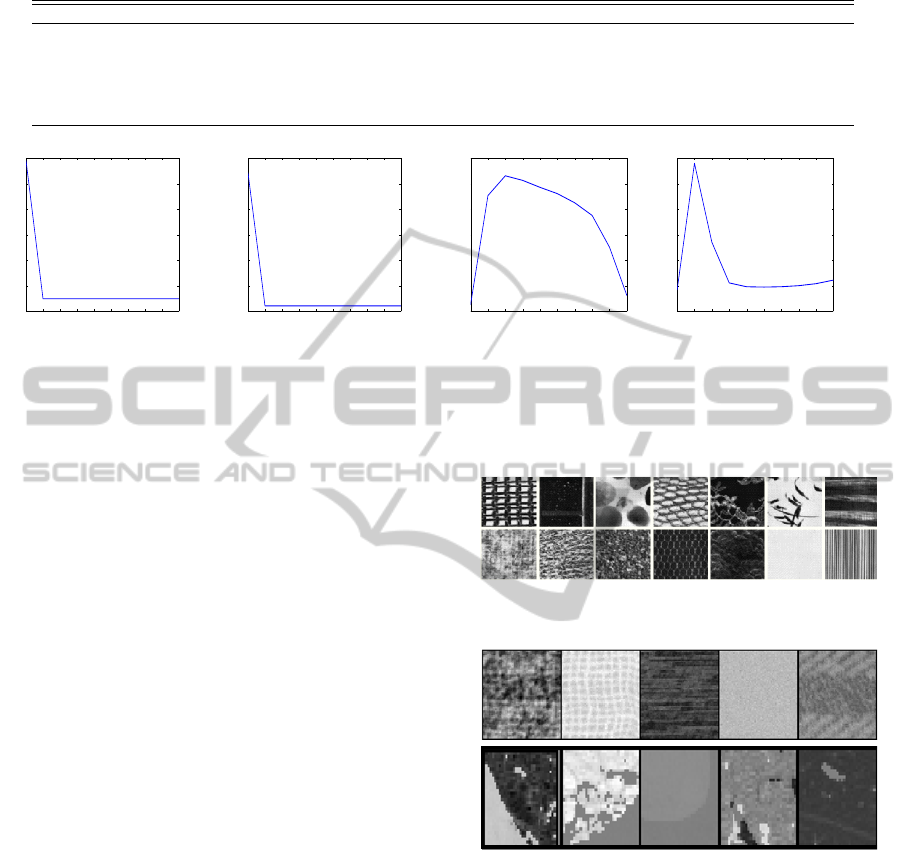
Table 1: Summary of classiﬁcation results attained by different classiﬁers on the Emphysema and Brodatz texture data sets.

Classiﬁer Emphysema Performance (Acc) Brodatz Performance (Acc)

k-Nearest Neighbour [Input=Image pixels, k=1] 46.04 ± 5.27% 29.06 ± 1.66%

Condensed Nearest Neighbour [Input=Image Pixels, 45% Data Retrieved | 25% Data Retrieved] 46.06 ± 5.19% 28.11 ± 2.01%

FK (Binary Binary RBM) [5 hid units] 47.31 ± 5.54% 16.81 ± 2.008%

FK (GaussianBinary RBM) [5 hidden units, σ = 1] 47.85 ± 4.83% 16.96 ± 2.40%

FK (Factored 3-Way RBM ) [5 hid units, 32 factors] 86.97 ± 5.54% 65 ± 4.6%

k-Nearest Neighbour [Input=Local Binary Pattern features, k=1] 95.2%(Sørensen et al., 2010) 91.4%(?)

1 2 3 4 5 6 7 8 9 10

4.469

4.47

4.471

4.472

4.473

4.474

4.475

x 10

No. of Epochs

Reconstruction Error

(a) RBM-BB(Emphysema)

1 2 3 4 5 6 7 8 9 10

4.3723

4.3724

4.3725

4.3726

4.3727

4.3728

4.3729

x 10

No. of Epochs

Reconstruction Error

(b) RBM-GB(Emphysema)

1 2 3 4 5 6 7 8 9 10

4.42

4.422

4.424

4.426

4.428

4.43

4.432

x 10

No. of Epochs

Reconstruction Error

sema)

1 2 3 4 5 6 7 8 9 10

2.81

2.815

2.82

2.825

2.83

2.835

2.84

x 10

No. of Epochs

Reconstruction Error

(d) Factored 3-Way RBM (Brodatz)

Figure 3: The reconstruction error shown after training different variants of RBM generative model on the Emphysema and

Brodatz data set for 10 epochs. The error for each of these models drops after several epochs; for factored 3-way model on

Emphysema, it ﬁrst rises, stabilises and then drops.

umn) and the reconstruction error for each model is

shown in Figure 3. Note that the best known perfor-

mance on Emphysema data set has been achieved by

(Sørensen et al., 2010), in which he used the leave one

subject out methodology to test the classiﬁer. Such

a partitioning scheme did not reveal discriminative

Fisher score space in our case, due to which we chose

holdout estimation method to train models and draw

Fisher scores. Consequently, the Fisher kernel de-

rived from factored 3-way RBM does give competi-

tive classiﬁcation performance in the same league as

shown by (Sørensen et al., 2010).

5.2 Brodatz Texture Data Set

The Brodatz textures (Valkealahti and Oja, 1998)

data set consists of a subset of 32 different classes

chosen randomly from the main Brodatz data set.

These textures are histogram equalized and then 20

patches

of size 64 × 64 are drawn from random lo-

cations of each class database for further experimen-

tation. Table 1 shows the classiﬁcation performance

of distance based approaches, i.e. k-NN and con-

densed NN on these preprocessed patches. The same

patches are also fed to the generative probability mod-

els for representational learning. Once the models

(binary-binary, gaussian-binary and factored 3-way)

are trained, a Fisher kernel is extracted from them and

then embedded into the SVM classiﬁer. The SVM

classiﬁes these textures using one versus one train-

ing of the gradients learnt by different models. The

hyperparameter C in SVM is once again decided via

Figure 4: Samples of texture images from the Brodatz data

set.

Figure 5: The visual factor ﬁlters, C

i f

learnt from the 64 ×

64 size patches of Brodatz data set (1

row) and 31 × 31

size patches of Emphysema data set (2

row).

grid search method. From the results obtained, we

observe that the Fisher kernel derived from a fac-

tored 3-way RBM gives better classiﬁcation perfor-

mance in comparison to the other Fisher kernel based

approaches and distance based classiﬁers on prepro-

cessed images. The best performance on the data set

is once again shown by local binary pattern features

classiﬁed through k-NN and shown in Table 1.

VISAPP2014-InternationalConferenceonComputerVisionTheoryandApplications

688

6 DISCUSSION AND FUTURE

WORK

In this paper, we present a novel approach of deriv-

ing a suitable classiﬁer for texture classiﬁcation that

uses the gradients of the generative model to differ-

entiate between different categories of textures. From

the experiments conducted above, we observed that

the performance of the Fisher kernel approach re-

lies on the discriminative quality of the Fisher score

space attained via maximum likelihood training of

the generative models. On a comparative scale, the

factored 3-way RBM proves better than the GBRBM

and BBRBM since it was able to provide less sparse

Fisher vectors that makes them suitable for discrimi-

nation in the dot product space. The dot product space

is not suitable for learning distance metric similarities

over sparse data, therefore Fisher vectors with zero or

very small gradients donot provide a space discrimi-

nant enough for texture classiﬁcation, as revealed for

FK-BBRBM and FK-GBRBM in Table 1. It is also

important to note that despite the availability of less

sparse Fisher vectors, the Fisher kernel classiﬁcation

performance still does not beat the best known clas-

siﬁcation performance on the Brodatz data set. This

follows us to the conclusion that a generative model

which is trained well via maximum likelihood learn-

ing does not necessarily give rise to a representation

that is well suited for classiﬁcation tasks. In practice,

the Fisher vectors for objects that have high proba-

bility under the model, will comprise of very small

gradients that are less likely to form a discriminative

basis for kernel functions. We would like to explore

this in more detail by overcoming the gradient scaling

problem through kernel normalization techniques in

the future. Such a kernel should satisfy the rationale

of achieving a discriminant Fisher score space by as-

signing similar gradients to two similar objects, and

maintaining inter-class separability too. The impact

of generative model’s scale on the Fisher score space

is also worth studying and will be pursued in future.

REFERENCES

Azim, T. and Niranjan, M. (2013). Inducing Discrimina-

tion in Biologically Inspired Models of Visual Scene

Recognition. In MLSP.

Chen, J., Kellokumpu, V., and Pietikinen, G. Z. . M. (2013).

RLBP: Robust Local Binary Pattern. In BMVC 2013,

Bristol, UK.

Cho, K., Alexander, A., and R.Tapani (2011). Improved

Learning of Gaussian-Bernoulli Restricted Boltzmann

Machines. In ANN - Volume Part I, ICANN, pages

1017, Berlin, Heidelberg. Springer-Verlag.

Cristani, M., Bicego, M., and Murino, V. (2002). Inte-

grated Region and Pixel Based Approach to Back-

ground Modelling. In Workshop on MVC, pages 3–8.

Hangarge, M., Santosh, K., Doddamani, S., and Pardeshi,

R. (2013). Statistical Texture Features Based Hand-

written and Printed Text Classiﬁcation in South Indian

Documents. CoRR, 1(32).

Haralick, R., Shanmugam, K., and Dinstein, I. (1973).

Textural Features for Image Classiﬁcation. SMC,

3(6):610–621.

Hinton, G. (2002). Training Products of Experts by Mini-

mizing Contrastive Divergence. Neural Computation,

14:1771–1800.

Hinton, G. and Salakhutdinov, R. (2009). Semantic Hash-

ing. IJAR, 50(7):969–978.

Jaakkola, T. and Haussler, D. (1999). Exploiting Genera-

tive Models in Discriminative Classiﬁers. NIPS, pages

487–493.

Kivinen, J. and Williams, C. (2012). Multiple Texture

Boltzmann Machines. In AISTATS, volume 22, pages

638–646.

Krizhevsky, A. (2009). Learning Multiple Layers of Fea-

tures from Tiny Images. Master’s thesis.

Marr, D. and Vaina, L. (1982). Representation and Recog-

nition of the Movements of Shapes. Proceedings of

the Royal Society of London. Series B. Biological Sci-

ences, 214(1197):501524.

Matheron, G. (1967). Representation and Recognition

of the Movements of Shapes. Proceedings of the

Royal Society of London. Series B. Biological Sci-

ences, 214(1197):501–524.

Mohamed, A., Dahl, G., and Hinton, G. (2010). Deep Belief

Networks for Phone Recognition. In NIPS.

Neal, R. (1996). Bayesian Learning for Neural Networks.

Springer-Verlag New York, Inc., Secaucus, NJ, USA.

Poggio, T., Voorhees, H., and Yuille, A. (1988). A Regular-

ized Solution to Edge Detection. Journal of Complex-

ity, 4(2):106 123

Ranzato, M., Krizhevsky, A., and Hinton, G. (2010).

Factored 3-Way Restricted Boltzmann Machines for

Modeling Natural Images. In AISTATS.

Serra, J. (1983). Image Analysis and Mathematical Mor-

phology. Academic Press, Inc., Orlando, FL, USA.

Sørensen, L., Shaker, S., and de Bruijne, M. (2010). Quan-

titative Analysis of Pulmonary Emphysema Using Lo-

cal Binary Patterns. Medical Imaging, 29(2):559–569.

Taylor, J. and Cristianini, N. (2004). Kernel Methods for

Pattern Analysis. Cambridge University Press, New

York, USA.

Tomita, F. and Tsuji, S. (1990). Computer Analysis of Vi-

sual Textures. Kluwer Academic Publishers, Norwell,

MA, USA.

Tuceryan, M. and Jain, A. (1998). Handbook of Pattern

Recognition & Computer Vision. Chapter Texture

Analysis, pages 235276. River Edge, NJ, USA

Valkealahti, K. and Oja, E. (1998). Reduced Multidimen-

sional Co-occurrence Histograms in Texture Classiﬁ-

cation. PAMI, 20(1):90–94.

TextureClassificationwithFisherKernelExtractedfromtheContinuousModelsofRBM

689

Weszka, J., Dyer, C., and Rosenfeld, A. (1976). A Compar-

ative Study of Texture Measures for Terrain Classiﬁ-

cation. SMC, 6(4):269–285.

Zhang, Y., X. Jian and J. Han (2005). Texture Feature-based

Image Classiﬁcation Using Wavelet Package Trans-

form. In AIC, volume 3644 of LNCS, pages 165 173.

Springer Berlin Heidelberg.

VISAPP2014-InternationalConferenceonComputerVisionTheoryandApplications

690