Statistical Methodology for Approximating G/G/1 Queues

by the Strong Stability Technique

Aicha Bareche and Djamil A

ıssani

Laboratory of Modeling and Optimization of Systems (LAMOS), University of B

eja

ıa, B

eja

ıa, Algeria

Keywords:

Queueing Systems, Strong Stability, Approximation, Boundary Density Estimation, Student Test, Simulation.

Abstract:

We consider a statistical methodology for the study of the strong stability of the M/G/1 queueing system

after disrupting the arrival ﬂow. More precisely, we use nonparametric density estimation with boundary

correction techniques and the statistical Student test to approximate the G/G/1 system by the M/G/1 one,

when the general arrivals law G in the G/G/1 system is unknown. By elaborating an appropriate algorithm,

we effectuate simulation studies to provide the proximity error between the corresponding arrival distributions

of the quoted systems, the approximation error on their stationary distributions and conﬁdence intervals for

the difference between their corresponding characteristics.

1 INTRODUCTION

In queueing theory performance evaluation may be

challenging task, for example, in the G/G/1 queue-

ing system, the Laplace transform and the generation

function are not available in closed form (Kleinrock,

1975). For this reason there exists, when a practi-

cal study is performed in queueing theory, a common

technique for substituting the real but complicated el-

ements governing a queueing system by simpler ones

in some sense close to the real elements. The queue-

ing model so constructed represents an idealization of

the real queueing one, and hence the stability prob-

lem arises. The stability problem in queueing theory

is concerned with the domain within which the ideal

queueing model may be taken as a good approxima-

tion of the real queueing system under consideration.

In other words, we clarify the conditions for which

the proximity in one way or another of the parameters

of the system involves the proximity of the studied

characteristics.

On the other hand, note that in practice all model

parameters are imprecisely known because they are

obtained by means of statistical methods. Such cir-

cumstances suggest to seek qualitative properties of

the real system, i.e., the manner in which the system

is affected by the changes in its parameters. These

qualitative properties include invariance, monotonic-

ity and stability. Its by means of qualitative properties

that bounds can be obtained mathematically and ap-

proximations can be made rigorously (Stoyan, 1983).

Even if the concept of stability is the same in a

general way, several approaches of the problem have

been elaborated. This led to the diversity of the deﬁ-

nitions and the methods of stability (Borovkov, 1984;

Rachev, 1989). Moreover, there is a signiﬁcant body

of literature on perturbation bounds of Markov chains.

One group of results uses the series expansion ap-

proach and the methods of matrix analysis (Heider-

gott and Hordijk, 2003; Heidergott et al., 2007). An-

other group employs the theory of operators and prob-

abilistic methods (A

ıssani and Kartashov, 1983; Kar-

tashov, 1996; Rachev, 1989).

In this work we will place more emphasis on the

strong stability method (A

ıssani and Kartashov, 1983;

Kartashov, 1996) which allows us to make both quali-

tative and quantitative analysis helpful in understand-

ing complicated models by more simpler ones for

which an evaluation can be made. This method, also

called ”method of operators” can be used to inves-

tigate the ergodicity and stability of the stationary

and non-stationary characteristics of the imbedded

Markov chains (A

ıssani and Kartashov, 1984; Kar-

tashov, 1996). In contrast to other methods, it sup-

poses that the perturbations of the transition kernel

are small with respect to some norms in the operators

space. This stringent condition gives better stability

estimates and enables us to ﬁnd precise asymptotic

expansions of the characteristics of the perturbed sys-

tem.

Note that the ﬁrst attempt to ”measure” the perfor-

mance of the strong stability method has been used

241

Bareche A. and Aïssani D..

Statistical Methodology for Approximating G/G/1 Queues by the Strong Stability Technique.

DOI: 10.5220/0004834002410248

In Proceedings of the 3rd International Conference on Operations Research and Enterprise Systems (ICORES-2014), pages 241-248

ISBN: 978-989-758-017-8

 2014 SCITEPRESS (Science and Technology Publications, Lda.)

in practice, and has been particularly applied to a

simple system of queues (Bouallouche and A

ıssani,

2006; Bouallouche and A

ıssani, ). The approach pro-

posed is based on the classical approximation method

where the authors perform the numerical proximity

of the stationary distribution of an Hyp/M/1 (respec-

tively M/Cox2/1) system by the one of an M/M/1

system when applying the strong stability method.

For the ﬁrst time, Bareche and A

ıssani (Bareche and

ıssani, 2008) specify an approximation error on the

stationary distributions of the G/M/1 (resp. M/G/1)

and M/M/1 systems when the general law of ar-

rivals (resp. service times) G is unknown and its den-

sity function is estimated by using the kernel density

method. In (Berdjoudj et al., 2012), the authors use

the discrete event simulation approach and the student

test to measure the performance of the strong stabil-

ity method through simple numerical examples for a

concrete case of queueing systems (the G/M/1 queue

after perturbation of the service law (Benaouicha and

ıssani, 2005), and the M/G/1 limit model for high

retrial intensities (which is the classical M/G/1 sys-

tem) after perturbation of the retrials parameter (Berd-

joudj and A

ıssani, 2003)). The same idea has been

already investigated for an approximation analysis of

the classical G/G/1 queue when the general law of

service is unknown and must be estimated by differ-

ent statistical methods, pointing out particularly the

impact of those taking into account the correction of

boundary effects (Bareche and A

ıssani, 2011), see

also the recent work of (Bareche and A

ıssani, 2013).

Indeed, note that in practice all model parameters

are imprecisely known because they are obtained by

means of statistical methods. In this sense, our con-

tribution concerns one aspect which is of some prac-

tical interest and has not sufﬁciently studied in the lit-

erature, for instance when a distribution governing a

queueing system is unknown and we resort to non-

parametric methods to estimate its density function.

Besides, as the strong stability method assumes that

the perturbation is small, then we suppose that the ar-

rivals law of the G/G/1 system is close to the expo-

nential one with parameter λ. This permits us to con-

sider the problem of boundary bias correction (Bouez-

marni and Scaillet, 2005; Chen, 2000; Schuster, 1985)

when performing nonparametric estimation of the un-

known density of the law G, since the exponential law

is deﬁned on the positive real line.

It is why we use, in this paper, the tools of

nonparametric density estimation to approximate the

complex G/G/1 system by the simpler M/G/1 one,

on the basis of the theoretical results addressed in

ıssani and Kartashov, 1984) involving the strong

stability of the M/G/1 system.

This article is organized as follows: In Section 2,

we describe the considered queueing models and we

present brieﬂy the strong stability of the M/G/1 sys-

tem. A review of boundary bias correction techniques

in nonparametric density estimation is given in Sec-

tion 3. The main new results of this paper are pre-

sented in Section 4, which shows the interest of com-

bining these nonparametric methods with the strong

stability principle for the study of the M/G/1 system.

It also points out the importance of using the Student

test to compare the characteristics of the two consid-

ered queueing systems, and presents a numerical case

study based on simulation results.

2 STRONG STABILITY OF THE

M/G/1 SYSTEM AFTER

PERTURBATION OF THE

ARRIVAL FLOW

2.1 Description of M/G/1 and G/G/1

Models

Consider a G/G/1 (FIFO, ∞) queueing system with

general service times distribution H and general inter-

arrival times probability distribution G. The following

notations are used: T

(the arrival time of the n

cus-

tomer), θ

(the departure time of the n

customer),

and γ

(the time till the arrival of the following cus-

tomer after θ

). Let us designate by ν

= ν(θ

+0) the

number of customers in the system immediately after

. ξ

represents the service time of the n

customer

arriving at the system. It is proved that X

= (ν

,γ

)

forms a homogeneous Markov chain with state space

N × R

and transition operator Q = (Q

i j

)

i, j≥0

, where

i j

(x,dy) = P(ν

n+1

= j, γ

n+1

∈ dy/ν

= i, γ

= x),

deﬁned by (see (A

ıssani and Kartashov, 1984)):

i j











(dy), if i = 0;

j−i

(x,dy), if i ≥ 1, j ≥ i;

p(x,dy), if j = i − 1, i ≥ 1;

0, otherwise;

(1)

where







(dy) =

P(T

≤ u < T

j+1

− u ∈ dy)dH(u);

(x,dy) =

∞

P(T

≤ u − x < T

j+1

− (u − x) ∈ dy)dH(u);

p(x,dy) =

P(x − u ∈ dy)dH(u).

Let us also consider an M/G/1 (FIFO,∞) sys-

tem and denote by E

the inter-arrivals distribution

is an exponential distribution with parameter λ),

and take the same distribution of service times than

the G/G/1 one. We introduce the corresponding fol-

lowing notations:

ν(

−0) and ξ

de-

ﬁned as above. The transition operator

Q =



i j



i, j>0

ICORES2014-InternationalConferenceonOperationsResearchandEnterpriseSystems

242

of the corresponding Markov chain

= (

) in

the M/G/1 system has the same form as in (1), where











(dy) = p

(dy), q

(x,dy) = p

(x)E

(dy),

p(x,dy) = p(x,dy);

exp(−λu)

(λu)

dH(u);

(x) =

∞

exp(−λ(u − x))

(λ(u−x))

dH(u).

Let us suppose that the arrival ﬂow of the G/G/1

system is close to the Poisson one. This proximity is

then characterized by the metric:

∗

= w

∗

(G,E

) =

∗

(t)|G − E

|(dt), (2)

where |a| designates the variation of the measure a

and ϕ

∗

is a weight function verifying the following

conditions:

• ϕ

∗

is non decreasing;

• ϕ

∗

(t + s) ≤ ϕ

∗

(t) · ϕ

∗

(s),∀t,s ∈ R

;

• ϕ

∗

(0) = 1.

We take ϕ

∗

(t) = e

δt

, with δ > 0. In addition, we use

the following notations:

∗

(t)E

(dt), (3)

∗

(t)G(dt), (4)

= w

(G,E

) =

|G − E

|(dt). (5)

2.2 Approximation of the G/G/1 System

by the M/G/1 One

In this section, we introduce some necessary no-

tations and recall the basic theorem of the strong

stability adapted to the studied case. For a general

framework see (A

ıssani and Kartashov, 1983; Kar-

tashov, 1996; Benaouicha and A

ıssani, 2005). In the

sequel, when no domain of integration is indicated,

an integral is extended over R

Consider the σ-algebra E , which represents the

product E

⊗ E

is the σ-algebra generated by

the countable partition of N and E

is the Borel

σ-algebra of R

We denote by mE the space of ﬁnite measures

on E , and we introduce the special family of norms

of the form kmk

∑

j≥0

v( j,y)|m

|(dy), ∀m ∈ mE ,

where v is a measurable function on N ×R

, bounded

below away from zero (not necessarily ﬁnite).

This norm induces a corresponding

norm in the space f E of bounded mea-

surable functions on N × R

, namely

k f k

= sup

k≥0

sup

x≥0

[v(k, x)]

−1

| f (k,x)|, ∀ f ∈

f E , as well as a norm in the space

of linear operators, namely kPk

sup

k≥0

sup

x≥0

[v(k, x)]

−1

∑

j≥0

v( j,y)|P

k j

(x,dy)|.

We associate to each transition kernel P the lin-

ear mapping P : f E → f E acting on f ∈ f E as

follows, (P f )(k,x) =

∑

j≥0

k j

(x,dy) f ( j,y). For

m ∈ mE and f ∈ f E the symbol m f denotes the

integral m f =

∑

j≥0

(dx) f ( j, x), and f ◦ m

denotes the transition kernel having the form

( f ◦ m)

i j

(x,A) = f (i,x)m

(A).

Remark 2.1. Using the norm deﬁned on the space

of ﬁnite measures introduced in the current section,

we can characterize the proximity of the two systems

G/G/1 and M/G/1 by

kG − E

∑

j≥0

+∞

v( j,t)|G − E

|(dt). (6)

Taking in (6), v( j,t) =



δt

, if j = 0,

0, if j 6= 0,

where δ > 0, one recovers the variational norm de-

ﬁned in (2).

Moreover, taking in (6), v( j,t) =



1, if j = 0,

0, if j 6= 0,

one recovers the variational norm deﬁned in (5).

Deﬁntion 2.1. (see (A

ıssani and Kartashov, 1983;

Kartashov, 1996)) A Markov chain X with transition

kernel P and invariant measure π is said to be strongly

υ-stable with respect to the norm k.k

, if kPk

< ∞

and each stochastic kernel Q in some neighborhood

{Q : kQ − Pk

< ε} has a unique invariant measure

µ = µ(Q) and kπ − µk

→ 0 as kQ − Pk

→ 0.

The following theorem determines the strong v-

stability conditions of the M/G/1 system after a small

perturbation of the arrivals law. It also gives the esti-

mates of the deviations of both the transition kernels

and the stationary distributions.

Theorem 2.1. (A

ıssani and Kartashov, 1984) Sup-

pose that in the M/G/1 system, the following ergod-

icity condition holds:

a) λ E(ξ) < 1; b) ∃a > 0 : E(e

aξ

) =

dH(u) < ∞,

where ξ is a random variable representing the service

times.

Suppose also that E

∗

< ∞ and β

= sup(β : H

∗

(λ −

λβ) < β), where H

∗

is the Laplace transform of the

probability density of the service times. Then, for all β

such that 1 < β < β

, the Markov chain X

is strongly

v−stable for the function v(n,t) = β

[exp(−αt) +

−1

∗

(t)], where:

α > 0, c =

βE

∗

1 − ρ

, and ρ =

∗

(λ − λβ) + β

2β

< 1.

In addition, if G

∗

< ∞, and w

≤

(β

−β)

, then we have

StatisticalMethodologyforApproximatingG/G/1Queues

bytheStrongStabilityTechnique

243

the margin between the transition operators:

kQ − Qk

≤ w

∗

(1 + β) + w

∗

(1 + λβ)

(β

− β)

where E

∗

and G

∗

are deﬁned respectively in (3) and

(4).

Moreover, if the general distribution of arrivals G is

such that:

∗

(G,E

) ≤

1 − ρ

(1 + c)

(1 + β + c

)

−1

(G,E

) ≤

(β

− β)

we obtain the deviation between the stationary dis-

tributions π and

π associated, respectively, to the

Markov chains X

and

, given by:

Er := kπ−πk ≤ 2[(1+β)w

∗

(1+c), (7)

where c

, c

are deﬁned as follows:

≤ c

where c

= 1 +

(1 − λm)(β− 1)(2 − ρ)E

∗

2(1 − ρ)

and m = E(ξ),

= G

∗

(1 + λβ)

(β

− β)

(1 − λm)(β − 1)(2 − ρ)

2(1 − ρ)β

Remark 2.2. The assumptions a) and b) of Theorem

2.1 imply the existence of a stationary distribution

for the imbedded Markov chain

in the M/G/1 sys-

tem. This distribution has the following form:

π({k}, A) =

(A) = p

(A), ∀ {k} ⊂ N and A ⊂ R

where p

= lim

n→∞

= k) = lim

t→∞

P(X(t) = k), where,

X(t) represents the size of the M/G/1 system at time

In general it is not possible to have stationary distri-

bution lim

t→∞

P(X(t) = k) of the M/G/1 system. How-

ever, one can compute its corresponding generating

function Π(z) given by (Kleinrock, 1975):

Π(z) = H

∗

(λ − λz)

(1 − ρ)(1 − z)

∗

(λ − λz)− z

, (8)

where ρ = λ E(ξ), H

∗

represents the Laplace trans-

form of the probability density of the service time ξ,

and z is a complex number verifying |z| ≤ 1. This for-

mula is called Pollaczek-Khinchin formula. Its inver-

sion allows us to ﬁnd the stationary distribution Π.

Formula (8) permits us to compute the stationary dis-

tribution of the queue length in a M/G/1 system. Un-

fortunately, for the G/G/1 system, this exact formula

is not known. So, if we suppose that the G/G/1 sys-

tem is close to the M/G/1 system, then we can use

formula (8) to approximate the G/G/1 system char-

acteristics with prior estimation of the corresponding

approximation error.

Given the bound in formula (7) in Theorem 2.1, it

remains to compute w

∗

and w

and methods to do so

will be discussed in the following.

3 BOUNDARY CORRECTION

TECHNIQUES IN

NONPARAMETRIC DENSITY

ESTIMATION

Different standard types of nonparametric density es-

timate are performed. For a survey, see the mono-

graph by Silverman (Silverman, 1986). The most

known and used nonparametric estimation method is

the kernel density estimate. If X

,..., X

is a sample

coming from a random variable X with probability

density function f and distribution F, then the Parzen-

Rosenblatt kernel estimator (Parzen, 1962; Rosen-

blatt, 1956) of the density f (x) for each point x ∈ R is

given by:

(x) =

∑

j=1

x − X

), (9)

where K is a symmetric density function called the

kernel and h

is the bandwidth.

Even if the choice of the kernel K is not of a great

importance, there would still remain the question of

which window width h

to choose. The problem of

bandwidth selection has been extensively studied (for

a survey, see (Jones et al., 1996)). The classical sym-

metric kernel estimate works well when estimating

densities with unbounded support. However, when

these latter are deﬁned on the positive real line [0,∞[,

without correction, the kernel estimates suffer from

boundary effects since they have a boundary bias (the

expected value of the standard kernel estimate at x = 0

converges to the half value of the underlying density

when f is twice continuously differentiable on its sup-

port [0,+∞) (Bouezmarni and Scaillet, 2005; Schus-

ter, 1985)). In fact, using a ﬁxed symmetric kernel

is not appropriate for ﬁtting densities with bounded

supports as a weight is given outside the support.

Several approaches have been introduced to get

a better estimation on the border. Some of them

proposed the use of particular kernels or bandwidths

(Schuster, 1985), other techniques propose the use

of estimators based on ﬂexible kernels (asymmetric

kernels (Bouezmarni and Scaillet, 2005; Chen, 2000)

and smoothed histograms (Bouezmarni and Scaillet,

2005)). They are very simple in implementation, free

of boundary bias, always nonnegative, their support

matches the support of the probability density func-

tion to be estimated, and their rate of convergence for

ICORES2014-InternationalConferenceonOperationsResearchandEnterpriseSystems

244

the mean integrated squared error is O(n

−4/5

). Below,

are brieﬂy discussed the estimators which we will use

in the context of this paper.

3.1 Reﬂection Method

Schuster (Schuster, 1985) suggests creating the mirror

image of the data in the other side of the boundary

and then applying the estimator (9) for the set of the

initial data and their reﬂection. f (x) is then estimated,

for x ≥ 0, as follows:

(x) =

∑

j=1

[K(

x − X

) + K(

x + X

)]. (10)

3.2 Asymmetric Gamma Kernel

Estimator

A simple idea for avoiding boundary effects is using

a ﬂexible kernel, which never assigns a weight out

of the support of the density function and which cor-

rects the boundary effects automatically and implic-

itly. The ﬁrst category of the ﬂexible kernels consists

of the asymmetric kernels (Bouezmarni and Scaillet,

2005; Chen, 2000) deﬁned by the form

(x) =

∑

i=1

K(x,b)(X

), (11)

where b is the bandwidth and the asymmetric kernel

K can be taken as a Gamma density K

with the pa-

rameters (x/b + 1,b) given by

(

+ 1,b)(t) =

x/b

−t/b

x/b+1

Γ(x/b + 1)

. (12)

3.3 Smoothed Histograms

The second category of ﬂexible kernels consists

of smoothed histograms (Bouezmarni and Scaillet,

2005) deﬁned by the form

(x) = k

+∞

∑

i=0

i,k

(x), (13)

where the random weights ω

i,k

are given by

i,k

= F

(

i + 1

) − F

(

where F

is the empiric distribution, k is the smooth-

ing parameter and p

(.) can be taken as a Poisson

distribution with parameter kx,

(x) = e

−kx

(kx)

, i = 0, 1,... (14)

4 STATISTICAL TECHNIQUES

FOR THE APPROXIMATION

OF THE G/G/1 SYSTEM BY

THE M/G/1 ONE

We want to apply nonparametric density estimation

methods to determine the variation distances w

and

∗

deﬁned respectively in (2) and (5), the proximity

error Er deﬁned in (7) between the stationary distri-

butions of the G/G/1 and M/G/1 systems and con-

ﬁdence intervals for the difference between the char-

acteristics of the considered systems in the stationary

state. We use the discrete event simulation approach

(Banks et al., 1996) to simulate the according systems

and we apply the Student test for the acceptance or

rejection of the equality of the corresponding charac-

teristics.

Note by Σ

and Σ

the G/G/1 and M/G/1 sys-

tems respectively. Let us repeat the simulation of the

system Σ

(i = 1,2) R

times. Note by θ

( j)

the theo-

retical value of the jth characteristic of Σ

. At the rth

repetition of the simulation of the system Σ

, one ob-

tains the estimate Y

( j)

of the characteristic θ

( j)

. Sup-

pose that the estimators Y

( j)

are unbiased. This im-

plies that θ

( j)

= E(Y

( j)

), r = 1,2,...,R

, i = 1,2.

For the comparison of the two queueing systems

and Σ

, we take the number of simulations R

= R large enough. With a signiﬁcance level α, the

conﬁdence interval for θ

( j)

− θ

( j)

is given by the fol-

lowing form:

( ¯y

( j)

− ¯y

( j)

) − t

(α/2 ; ν)

σ( ¯y

( j)

− ¯y

( j)

) ≤ θ

( j)

− θ

( j)

(15)

≤ ( ¯y

( j)

− ¯y

( j)

) + t

(α/2 ; ν)

σ( ¯y

( j)

− ¯y

( j)

where ¯y

( j)

∑

r=1

( j)

, i = 1,2, σ( ¯y

( j)

− ¯y

( j)

) is the

standard error of the punctual speciﬁed estimator, ν =

2(R − 1) is the number of degrees of freedom, and

(α/2 ; ν)

is a value to be taken on the Student table.

To take a decision on how signiﬁcant is the differ-

ence between the tow systems, we check if the con-

ﬁdence interval for θ

( j)

− θ

( j)

contains the zero value

or not. We have the following conclusions:

1. If the conﬁdence interval for θ

( j)

− θ

( j)

does not

contain the zero (i.e. it is totally on the left-hand

side or on the right-hand side of zero), then it is

extremely probable that θ

( j)

< θ

( j)

or θ

( j)

> θ

( j)

respectively.

2. If the conﬁdence interval for θ

( j)

− θ

( j)

contains

the zero, then there is no statistical obviousness

afﬁrming that the jth characteristic of one of the

systems is better than that of the other.

StatisticalMethodologyforApproximatingG/G/1Queues

bytheStrongStabilityTechnique

245

Table 1: Performance measures with different estimators.

g(x) g

(x) ˜g

(x) ˆg

(x)

Mean arrival rate λ 1.6874 1.5392 1.6503 1.6851 1.6840

Trafﬁc intensity of the system

0.1562 0.1578 0.1570 0.1564 0.1567

Variation distance w

0.0096 0.1287 0.0114 0.0102 0.0105

Variation distance w

∗

0.0183 0.2536 0.0311 0.0206 0.0224

Error on stationary distributions Er 0.0356 0.0452 0.0378 0.0377

In the context of this paper, we consider the fol-

lowing characteristics:

• ¯n

,i = 1,2, mean number of customers in the sys-

tem i.

•

,i = 1, 2, output rate in the system i.

•

,i = 1,2, sojourn mean time of a customer in the

system i (response time of the system).

•

,i = 1, 2, occupation rate of the system i.

To realize this work, we elaborated an algorithm

which follows the following steps:

1) Generation of a sample of size n of general ar-

rivals distribution G with theoretical density g(x).

2) Use of a nonparametric estimation method to es-

timate the theoretical density function g(x) by a

function denoted in general g

∗

(x).

3) Calculation of the mean arrival rate given by: λ =

xdG(x) = 1/

xg(x)dx = 1/

∗

(x)dx.

4) Veriﬁcation, in this case, of the strong stability

conditions given in the subsection 2.2. For calcu-

lation considerations, the variation distances w

and w

∗

are given respectively by: w

|G −

|(dx) '

∗

− e

|(x)dx and w

∗

δx

|G −

|(dx) '

δx

∗

− e

|(x)dx, where δ > 0.

5) Computation of the minimal error on the station-

ary distributions of the considered systems ac-

cording to (7).

6) Application of the Student test to determine the

difference between the corresponding character-

istics of the considered systems according to (15).

Simulation studies were performed under the Matlab

7.1 environment. The Epanechnikov kernel (Silver-

man, 1986) is used throughout for estimators involv-

ing symmetric kernels. The bandwidth h

is chosen

to minimize the criterion of the ”least squares cross-

validation” (Jones et al., 1996). The smoothing pa-

rameters b and k are chosen according to a bandwidth

selection method which leads to an asymptotically op-

timal window in the sense of minimizing L

distance

(Bouezmarni and Scaillet, 2005).

4.1 Simulation Study

We consider a G/G/1 system such that the gen-

eral inter-arrivals distribution G is assumed to be a

Gamma distribution with parameters α = 0.7, β = 2,

denoted Γ(0.7, 2), with a theoretical density g(x) and

the service times distribution is Cox2 with parame-

ters: µ

= 3, µ

= 10, a = 0.005.

By generating a sample coming from the Γ(0.7,2)

distribution, we use the different nonparametric esti-

mators given respectively in (9)-(14) to estimate the

theoretical density g(x)

For these estimators, we take the sample size n =

200 and the number of simulations R = 100. For

the construction of conﬁdence intervals using the Stu-

dent test, we take the signiﬁcance level α = 0.05.

Hence the number of degrees of freedom ν = 198 and

(α/2 ; ν)

= t

(0.025 ; 198)

= 1.96.

Curves of the theoretical and estimated densities

are illustrated in Figure 1. Different performance

measures are listed in Table 1.

The conﬁdence intervals are shown respectively

in Tables 2, 3, 4, 5 and 6, by giving their lower and

upper bounds.

Table 2: Conﬁdence intervals with theoretical density g(x).

Characteristics

difference

wer bound

Upper

bound

¯n

− ¯n

-0.0204 0.0098

−

-0.0120 0.0016

−

-0.0523 0.0273

−

-0.0087 0.0025

Table 3: Conﬁdence intervals with Parzen-Rosenblatt esti-

mator g

(x).

Characteristics

difference

wer bound

Upper

bound

¯n

− ¯n

-0.0394 -0.0120

−

-0.0305 -0.0106

−

-0.0923 -0.0416

−

-0.0637 -0.0398

Discussion: Figure 1 shows that the use of nonpara-

metric density estimation methods taking into account

the correction of boundary effects improves the qual-

ity of the estimation (compared to the curve of of the

Parzen-Rosenblatt estimator, those of mirror image,

asymmetric Gamma kernel and smoothed histogram

ICORES2014-InternationalConferenceonOperationsResearchandEnterpriseSystems

246

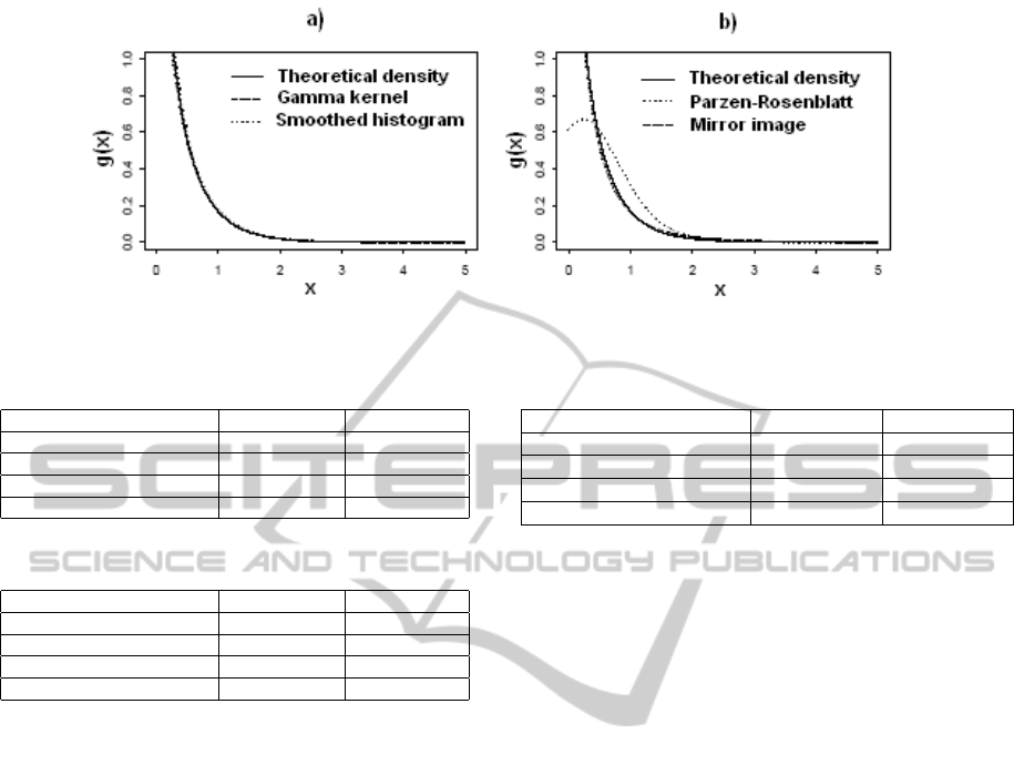
Figure 1: Theoretical density g(x) = Γ(0.7,2)(x), and estimated densities.

Table 4: Conﬁdence intervals with mirror image estimator

˜g

(x).

Characteristics dif

ference

Lower

bound

Upper bound

¯n

− ¯n

-0.0389 0.0089

−

-0.0314 0.0122

−

-0.0565 0.0697

−

-0.0128 0.0130

Table 5: Conﬁdence intervals with asymmetric Gamma ker-

nel estimator ˆg

(x).

Characteristics dif

ference

Lower

bound

Upper bound

¯n

− ¯n

-0.0213 0.0018

−

-0.0175 0.0019

−

-0.0379 0.0365

−

-0.0085 0.0027

estimators are closer to the curve of the theoretical

density). We note in Table 1 that the approximation

error on the stationary distributions of the G/G/1 and

M/G/1 systems was given when applying nonpara-

metric density estimation methods by considering the

correction of boundary effects such in the cases of us-

ing the mirror image estimator (Er = 0.0452), asym-

metric Gamma kernel estimator (Er = 0.0378) and

smoothed histogram (Er = 0.0377). In addition, these

two last errors are close to the one given when us-

ing the theoretical density g(x) (Er = 0.0356). But,

when applying the Parzen-Rosenblatt estimator which

does not take into account the correction of bound-

ary effects, the approximation error Er on the station-

ary distributions of the quoted systems could not be

given. This shows the importance of the smallness of

the proximity error of the two corresponding arrival

distributions of the considered systems, characterized

by the variation distances w

and w

∗

We notice also that in the cases of using the theo-

retical density g(x), the mirror image estimator ˜g

(x),

the Gamma kernel estimator ˆg

(x) and the smoothed

histogram ˆg

(x) , with a signiﬁcance level α = 0.05,

we do not reject any hypotheses since all the intervals

contain zero (see Tables 2, 4, 5 and 6). This means

that, with this level α = 0.05, the corresponding char-

Table 6: Conﬁdence intervals with smoothed histogram

ˆg

(x).

Characteristics difference Lower bound Upper bound

¯n

− ¯n

-0.0254 0.0012

−

-0.0138 0.0022

−

-0.0386 0.0296

−

-0.0092 0.0038

acteristics of the two considered systems are not sig-

niﬁcantly different. In addition, we remark that the

conﬁdence intervals are very close. That gives an idea

about the accuracy of the approximation. But in the

case of using the Parzen-Rosenblatt estimator g

(x),

with the same level α = 0.05, all the hypotheses are

rejected since all the intervals do not contain zero (see

Table 3). This means that the risk of wrongly reject-

ing these hypotheses is of order 5%. So, we prefer to

say that the corresponding characteristics of the two

systems considered are signiﬁcantly different.

The theoretical results (A

ıssani and Kartashov, 1984)

are then illustrated by numerical results. Indeed, it

is noted that in practice, for a low margin between

the service laws of the G/G/1 and M/G/1 queueing

systems, it is possible to approximate the G/G/1 sys-

tems characteristics with the corresponding ones of

the M/G/1 system when the general distribution G

of arrivals is unknown and must be estimated. In ad-

dition, this approximation is as much accurate than

∗

and w

are small. Note also that contrary to non

parametric methods taking into account the boundary

bias correction, the classical kernel density estimate

is inappropriate for determining this type of approxi-

mation.

5 CONCLUSIONS AND FURTHER

RESEARCH

Simulation studies presented in this paper show the

importance of some aspects in the application of the

StatisticalMethodologyforApproximatingG/G/1Queues

bytheStrongStabilityTechnique

247

strong stability method to queueing systems. First of

all, the smallness of the perturbation done has a sig-

niﬁcant impact on the determination of the proximity

of the considered systems and hence on the approxi-

mation error on their stationary distributions. On the

other hand, when statistical methods are used to es-

timate an unknown density function in a considered

system, we cannot ignore the problem of boundary

effects.

To summarize, we show the interest of some sta-

tistical techniques (nonparametric estimation meth-

ods with boundary bias techniques and Student test)

to measure the performance of the strong stability

method in a M/G/1 queueing system after perturba-

tion of the arrival ﬂow. Indeed, we note that practi-

cally, for a low margin between the arrival laws of the

G/G/1 and M/G/1 systems, and by taking into ac-

count the boundary effects when using nonparametric

density estimation to estimate the unknown arrivals

law G in the G/G/1 system, it is possible to approx-

imate the G/G/1 system’s characteristics by the cor-

responding ones of the M/G/1 system.

A closely ﬁeld of practical interest can be de-

scribed as follows: when modeling insurance claims,

one could be interested in the loss distribution which

describes the probability distribution of payment to

the insured. It is a positive variable, hence the pres-

ence of the boundary bias problem. The asymmetric

Beta kernel estimates are suitable for estimating this

type of heavy-tailed distributions.

REFERENCES

ıssani, D. and Kartashov, N. (1983). Ergodicity and sta-

bility of Markov chains with respect to operator topol-

ogy in the space of transition kernels. Compte Rendu

Academy of Sciences U.S.S.R, ser., A 11:3–5.

ıssani, D. and Kartashov, N. (1984). Strong stability of the

imbedded Markov chain in an M/G/1 system. Theory

of Probability and Mathematical Statistics, American

Mathematical Society, 29:1–5.

Banks, J., Carson, J., and Nelson, B. (1996). Discrete-Event

System Simulation. Prentice Hall, New Jersey.

Bareche, A. and A

ıssani, D. (2008). Kernel density in the

study of the strong stability of the M/M/1 queueing

system. Operations Research Letters, 36 (5):535–538.

Bareche, A. and A

ıssani, D. (2011). Statistical techniques

for a numerical evaluation of the proximity of G/G/1

and G/M/1 queueing systems. Computers and Math-

ematics with Applications, 61 (5):1296–1304.

Bareche, A. and A

ıssani, D. (2013). Combinaison

des m

ethodes de stabilit

e forte et d’estimation non

param

etrique pour l’approximation de la ﬁle d’attente

G/G/1. Journal europ

een des syst

emes automatis

es,

47 (1-2-3):155–164.

Benaouicha, M. and A

ıssani, D. (2005). Strong stability

in a G/M/1 queueing system. Theor. Probability and

Math. Statist., 71:25–36.

Berdjoudj, L. and A

ıssani, D. (2003). Strong stability in

retrial queues. Theor. Probab. Math. Stat., 68:11–17.

Berdjoudj, L., Benaouicha, M., and A

ıssani, D. (2012).

Measure of performances of the strong stability

method. Mathematical and Computer Modelling,

56:241–246.

Borovkov, A. (1984). Asymptotic Methods in Queueing

Theory. Wiley, New York.

Bouallouche, L. and A

ıssani, D. Performance Analysis Ap-

proximation in a Queueing System of Type M/G/1.

Bouallouche, L. and A

ıssani, D. (2006). Measurement and

Performance of the Strong Stability Method. Theory

of Probability and Mathematical Statistics, American

Mathematical Society, 72:1–9.

Bouezmarni, T. and Scaillet, O. (2005). Consistency of

Asymmetric Kernel Density Estimators and Smoothed

Histograms with Application to Income Data. Econo-

metric Theory, 21:390–412.

Chen, S. X. (2000). Probability Density Function Estima-

tion Using Gamma Kernels. Ann. Inst. Statis. Math.,

52:471–480.

Heidergott, B. and Hordijk, A. (2003). Taylor expansions

for stationary markov chains. Adv. Appl. Probab.,

35:1046–1070.

Heidergott, B., Hordijk, A., and Uitert, M. V. (2007). Series

expansions for ﬁnite-state markov chains. Adv. Appl.

Probab., 21:381–400.

Jones, M. C., Marron, J. S., and Sheather, S. J. (1996). A

brief survey of bandwidth selection for density esti-

mation. J.A.S.A., 91:401–407.

Kartashov, N. V. (1996). Strong Stable Markov Chains.

TbiMC Scientiﬁc Publishers, VSPV, Utrecht.

Kleinrock, L. (1975). Queueing Systems, vol. 1. John Wiley

and Sons.

Parzen, E. (1962). On estimation of a probability density

function and mode. Ann. Math. Stat., 33:1065–1076.

Rachev, S. (1989). The problem of stability in queueing

theory. Queueing Systems, 4:287318.

Rosenblatt, M. (1956). Remarks on some non-parametric

estimates of a density function. Ann. Math. Statist.,

27:832–837.

Schuster, E. F. (1985). Incorporating support constraints

into nonparametric estimation of densities. Commun.

Statist. Theory Meth., 14:1123–1136.

Silverman, B. W. (1986). Density Estimation for Statistics

and Data Analysis. Chapman and Hall, London.

Stoyan, D. (1983). Comparison Methods for Queues and

Other Stochastic Models (English translation). In:

Daley, D.J. (Ed.), Wiley, New York.

ICORES2014-InternationalConferenceonOperationsResearchandEnterpriseSystems

248