Curve Reconstruction from Noisy and Unordered Samples

Marek W. Rupniewski

Institute of Electronic Systems, Warsaw University of Technology, Nowowiejska 15/19, 00-665 Warsaw, Poland

Keywords:

Curve Reconstruction, Noisy Samples.

Abstract:

An algorithm for the reconstruction of closed and open curves from clouds of their noisy and unordered

samples is presented. Each curve is reconstructed as a polygonal path represented by its vertices, which

are determined in an iterative process comprising evolutionary and decimation stages. The quality of the

reconstruction is studied with respect to the local density of the samples and the standard deviation of the

noise perturbing the samples. The algorithm is veriﬁed to work for arbitrary dimensions of ambient space.

1 INTRODUCTION

In many engineering problems, there is a need to ﬁt

a curve to an irregularly spaced set of points. Typ-

ically, these problems fall into one of the following

categories. If the ordered points lie exactly on the

curve to be found, then one deals with an interpo-

lation problem. If the points still lie on the curve,

but their order on the curve is unknown, then one

must recover the order prior to interpolation. For this

task, one may use e.g. the algorithms presented in

(Gold and Snoeyink, 2001), (Dey et al., 2000), (Al-

thaus and Mehlhorn, 2001). If one knows the order

of the points along the curve, but the points are dis-

turbed by the noise, then one approximates the curve

usually with some kind of splines, see e.g. (Co-

hen and O’Dell, 1989), (Fritsch and Carlson, 1980),

(H¨olzle, 1983). Finally, one may face a problem

where both the noise is present, and the order of the

sample points along the curve is unknown. This kind

of problem appears in Computed Axial Tomography

(CAT), Coordinate-Measuring Machine (CMM) mea-

surements and Magnetic Resonance Imaging (MRI).

In the literature, there are given various strategies to

solve the problems falling into this class. Fang and

Gossard (Fang and Gossard, 1995) proposed ﬁtting

a curve with given end-points by minimizing some

spring energy function. Goshtasby (Goshtasby, 2000)

obtained a reconstruction by tracing ridges of a cer-

tain inverse distance function (for this, he needed

to evaluate the function on a dense grid). A pixel-

based solution was proposed by Pottmann and Ran-

drup (Pottmann and Randrup, 1998). They recovered

a curve as a medieval line of a set of pixels (of appro-

priate size) that cover the points. There is also an ap-

proach to the problem based on moving least-square

method showed by Levin (Levin, 1998) and improved

by Lee (Lee, 2000). A more statistic point of view

led Hastie and Stuetzle (Hastie and Stuetzle, 1989)

towards the reconstruction of the unknown curve as

a principal curve of the given set of points. Finally,

let us mention the work of Cheng et al. (Cheng et al.,

2005) in which a curve was reconstructed by deter-

mining and following a minimum width strip contain-

ing the noisy points.

The way we solve the problem of curve recon-

struction starts with a choice of a number of balls cen-

tered at the curve samples. Then, in each iteration,

the balls are moved (hopefully towards the original

curve) and their number is reduced in such a way that

they do not overlap too much. Eventually, the balls’

centers are ordered and then claimed to be consecu-

tive vertices of a polygonal path approximating the

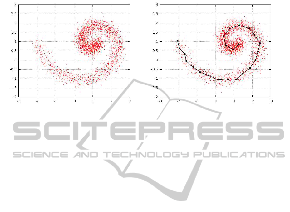
curve being recovered (see Fig. 1 for an example of

the cloud of samples and a result of the reconstruc-

tion algorithm).

The obtained polygonalpath, being an approxima-

tion itself, may also play a role of an “initial guess”

that is fundamental for the success of more sophisti-

cated reconstruction algorithms (see e.g. (Ruiz et al.,

2013)). One may also use the obtained vertices for

construction of a smooth, instead of a polygonal, ap-

proximation based, for example, on splines or rational

Gaussian curves (Goshtasby, 1995).

183

W. Rupniewski M..

Curve Reconstruction from Noisy and Unordered Samples.

DOI: 10.5220/0004814801830188

In Proceedings of the 3rd International Conference on Pattern Recognition Applications and Methods (ICPRAM-2014), pages 183-188

ISBN: 978-989-758-018-5

 2014 SCITEPRESS (Science and Technology Publications, Lda.)

(a) (b)

Figure 1: A set D of noisy samples of an unknown curve (Subﬁg. 1(a)) and a reconstruction (solid line on Subﬁg. 1(b))

resulted from D.

2 PROBLEM STATEMENT

The aim is to recover a piece-wise smooth curve

γ ⊂ R

given a set of curve samples that are affected

by some noise. We will assume that the samples

are independent, i.e. that they form a set D of re-

alizations of identically distributed and independent

random variables with some probability density func-

tion f : R

→ R , which has its support located along

curve γ.

By recovering curve γ from set D we mean con-

structing a polygonal path (determined by the se-

quence of its vertices) that approximates γ. The qual-

ity of this approximation may be assessed by the

Hausdorff distance d between the polygonal path

and curve γ:

d(γ,

γ) = max



max

p∈γ

min

q∈

kp − qk, max

p∈

min

q∈γ

kp − qk



Of course to perform such an assessment one needs

to know γ, which is rarely the case except for simula-

tions.

The quality of curve reconstruction depends upon

many factors:

• the number of samples n,

• their distribution along curve γ,

• the distribution of sample errors,

• the dimension d of the ambient space R

• the curvature of the curve.

In section 4, the quality of the reconstruction is stud-

ied in the case of uniform distribution of the samples

with respect to the arc length of the curve, normal

distribution of the sample errors and negligible cur-

vature.

3 ALGORITHM

The algorithm for curve reconstruction consists of

four steps (two of which are repeated in a loop) and is

presented in Fig. 2. The result of the algorithm is a set

E of pairs of the end-points of line segments compris-

ing a polygonal path approximating the curve.

Require: a non-empty set D ⊂ R

of noisy samples

of an unknown curve γ and a parameter R > 0

S ← choose(D, R)

repeat

S ← evolve(S, D, R)

S ← decimate(S, R)

until S is not affected by the last decimation

E ← order(S, R)

Figure 2: The algorithm for curve reconstruction.

3.1 Initialization

In the ﬁrst step of the algorithm

S ← choose(D, R)

an initial set S of the path’s nodes is chosen. For

simplicity, we propose taking for S a randomly cho-

sen R-separated subset of the sample set D, where by

R-separated set we mean a set having no two different

points closer than R.

ICPRAM2014-InternationalConferenceonPatternRecognitionApplicationsandMethods

184

3.2 Evolution

The heart of the curve reconstruction algorithm is the

evolution of the set S

S ← evolve(S, D, R).

The aim of the evolution is to move the points be-

longing to S towards the curve being reconstructed

and spread them along this curve. The evolution al-

gorithm is presented in Fig. 3.

repeat

Q ← S

S ← {avg(D∩ vcell(p, Q, R)) | p ∈ Q}

until Q = S

Figure 3: Function Q = evolve(S, D, R). avg(X) denotes the

mass centre of the points from X ⊂ R

In each step of the evolution, every node p ∈ S is

moved to the mass centre of the points from D falling

into the intersection vcell(p, S, R) of the ball of radius

R centered at p and the p’s cell of the Voronoi diagram

constructed for S, i.e.,

vcell(p, S, R) =

q ∈ R

|∀

o∈S

R ≥ kp − qk ≤ kp − ok

, (1)

where kxk denotes the Euclidean norm of x ∈ R

. In

Fig. 4 an example of the four-point node set is pre-

sented and the related intersections are depicted with

various gray levels.

Figure 4: The cells (see eq. (1)) constructed for a four-point

node set S. Each cell is the intersection of a ball centered at

a point, and this point’s Voronoi cell of the Voronoi diagram

constructed for S.

Moving a point towards the mass center of its

small circular neighbourhood accounts for conver-

gence towards the region of bigger mass density (we

assume that the closer is a point to the curve being

reconstructed, the bigger is the probability of hav-

ing a sample falling into the neighbourhood of the

point). Restricting the circular neighbourhoods to the

Voronoi cells prevents the points from concentrating

around single points of the curve.

while #S > 3 and there are points p ∈ S satisfying

condition (2) do

remove from S a randomly chosen point p satis-

fying (2)

end while

Figure 5: Function S ← decimate(S, R).

3.3 Decimation

The decimation step

S ← decimate(S, R)

of the algorithm is responsible for the reduction of the

number of points in S. Thus, it directly affects the rate

of convergence of the algorithm, the robustness of the

algorithm with respect to outliers, and the ability of

the algorithm to cope with curve self-intersections, its

end-points, and other singularities (in case there are

any).

In this paper, we present an algorithm for recon-

struction of smooth curves without self-intersections.

Therefore, we propose quite a simple decimation al-

gorithm presented in Fig. 5. In its formulation, the

statement that p ∈ S satisﬁes condition (2) means

that p has more than two other points from S in its

2R-neighbourhood or it has less than two other points

from S in its 4R-neighbourhood, i.e.,

#{q ∈ S|kp− qk ≤ 2R} > 3 or

#{q ∈ S|kp− qk ≤ 4R} < 3. (2)

3.4 Ordering

During the ordering step

E ← order(S, R)

the points belonging to set S are ordered so that two

consecutive points on the polygonal path are consec-

utive in sequence E. One can think of this stage as of

joining points of S with line segments in order to ob-

tain a polygonal path (open or closed). A line segment

may be represented with the set of its two end-points.

The algorithm for identifying all such segments is pre-

sented in Fig. 6. The algorithm is designed so that it

can produce more than one path in case the samples

origin from more than one curve.

4 SIMULATION

To asses the quality of the reconstruction algorithm

the following simulations were performed. Samples

CurveReconstructionfromNoisyandUnorderedSamples

185

E ← {{p, q} ⊂ S | p 6= q and kp − qk ≤ 2R}

while there are points p, q ∈ S such that each of

them appears in at most one pair comprising set E

and kp− qk ≤ 4R do

E ← E ∪



{p, q}



end while

Figure 6: Function E ← order(S, R).

of a line segment I = [0, 100] × {0} ⊂ R

were cho-

sen according to uniform distribution, and then they

were perturbed by standard normal deviates. Please

note that this is also a model for situation, in which

the original curve has some non-zero curvature but

the radius of this curvature is much bigger than the

standard deviation of the noise (locally, after proper

scaling, the curve looks like a line segment and the

deviates become standard). For various values of the

algorithm parameter R and for various number ρ of

samples per unit length line segment, the following

outputs of the algorithm were gathered:

• the median of the distances between the polygonal

path vertices and line segment I,

• the maximum of the distances between the polyg-

onal path vertices and line segment I,

• the bigger of the distances between the polygonal

path and the end-points of I.

The maximum of the latter two quantities forms the

Hausdorff distance between polygonal path and the

line segment being reconstructed. The experiments

were repeated 100 times for each set of parameters

in order to estimate the mean value and the quartiles

for the above quantities. The results are presented in

Fig. 8.

According to this ﬁgure, for a given number of

samples (per unit length curve segment) and the devi-

ation of the noise, the radius R should be neither too

small nor too big. The small values of R do not allow

points of S to evolve towards the segment, while the

big values of R results in worse approximation of the

end-points of the segment. We can also observe that

the distance between the polygonal path vertices and

the line segment decrease with the number of sam-

ples (this decrease is almost linear for big numbers of

samples), while the distance from these vertices to the

end-points of the segment tends to a non-zero value

that depends on parameter R.

4.1 Higher Dimensions

To verify that the algorithm produces desired results

for dimensions of the ambient space bigger than two,

another set of experiments was conducted. Samples

(a)

(b)

Figure 7: Results of reconstructions of a line segment ly-

ing in a d-dimensional space. Subﬁg. 7(a) shows estimated

quartiles and median distance between reconstructed polyg-

onal path vertices and the line segment. The median is de-

picted with a solid line, while the lower and the upper quar-

tiles are shown with the dashed lines. Subﬁg. 7(b) shows

estimates of the bigger of the two distances between an end-

point of the segment and the set of the path vertices. In the

both cases σ denotes the standard deviation of the normal

noise perturbing the samples.

of a line segment

I = [0, 100] × {0}

d−1

⊂ R

were perturbed by standard normal deviates. The pa-

rameter R of the reconstruction algorithm was ﬁxed,

and a number of reconstructions were performed for

various values of the dimension d and various densi-

ties ρ of samples per unit length line segment. The

resulting characteristics are shown in Fig. 7.

ICPRAM2014-InternationalConferenceonPatternRecognitionApplicationsandMethods

186

(a) (b)

(e) (f)

Figure 8: Results of reconstructions of a line segment (lying in R

) from its samples disturbed by normal deviates with

standard deviation σ. ρ stands for mean number of samples per unit length line segment. In Subﬁg. 8(a) and 8(b) the estimated

median distance from polygonal path vertices to the segment is shown. In Subﬁg. 8(c) and 8(d) the estimated maximum of the

same distance is presented. The last two subﬁgures show estimates of the bigger of the two distances between an end-point

of the segment and the set of polygonal path vertices. In each ﬁgure, dashed lines show the lower and the upper estimated

quartiles for the corresponding (by color) quantity.

CurveReconstructionfromNoisyandUnorderedSamples

187

5 APPLICATION

The presented algorithm has been successfully used

for the purpose of air targets trajectory reconstruction

from radar raw data. The data comprised range bins

at which the recorded signal exceeded a given thresh-

old. The original data and the result of trajectory re-

construction are presented in Fig. 9.

Figure 9: Air target reconstruction from raw radar data (the

axes are scaled in kilometers; the right Figure was obtained

with the algorithm for R = 0.9km).

6 CONCLUSIONS

In this paper we have presented a novel algorithm for

the reconstruction of a curve from a cloud of its noisy

and unordered samples. One of the merits of the al-

gorithm is its simplicity – others include:

• no requirement of an initial guess for the recon-

structed curve,

• the curve end-points don’t need to be speciﬁed,

• it ambient space dimension is arbitrary,

• it works for both open and closed curves,

• it works for any number of disjoint curves.

The algorithm, in its presented form, does not cope

with intersecting curves well. Research is being un-

dertaken to improve it in this aspect. Also, we are

working on adapting the algorithm to anisotropic data

(e.g., location-time data points) and on automatic

adaptation of parameter R.

ACKNOWLEDGEMENTS

This work has been supported by the National Center

for Research and Development (NCBiR) under Grant

No. DOBR/0041/R/ID1/2012/03.

REFERENCES

Althaus, E. and Mehlhorn, K. (2001). Traveling salesman-

based curve reconstruction in polynomial time. SIAM

Journal on Computing, 31(1):27–66.

Cheng, S.-W., Funke, S., Golin, M., Kumar, P., Poon, S.-

H., and Ramos, E. (2005). Curve reconstruction from

noisy samples. Computational Geometry, 31(12):63 –

100.

Cohen, E. and O’Dell, C. (1989). A data dependent

parametrization for spline approximation. Mathemat-

ical Methods in Computer Aided Geometric Design,

pages 155–166.

Dey, T., Mehlhorn, K., and Ramos, E. (2000). Curve

reconstruction: Connecting dots with good reason.

Computational Geometry: Theory and Applications,

15(4):229–244.

Fang, L. and Gossard, D. C. (1995). Multidimensional

curve ﬁtting to unorganized data points by nonlinear

minimization. Computer-Aided Design, 27(1):48 –

58.

Fritsch, F. and Carlson, R. (1980). Monotone piecewise

cubic interpolation. SIAM J. Numer. Anal., 17(2):238–

246.

Gold, C. and Snoeyink, J. (2001). A one-step crust and

skeleton extraction algorithm. Algorithmica (New

York), 30(2):144–163.

Goshtasby, A. (1995). Geometric modelling using rational

gaussian curves and surfaces. Computer-Aided De-

sign, 27(5):363 – 375.

Goshtasby, A. (2000). Grouping and parameterizing irreg-

ularly spaced points for curve ﬁtting. ACM Transac-

tions on Graphics, 19(3):185–203.

Hastie, T. and Stuetzle, W. (1989). Principal curves. Journal

of the American Statistical Association, 84(406):502–

516.

H¨olzle, G. (1983). Knot placement for piecewise polyno-

mial approximation of curves. Computer-Aided De-

sign, 15(5):295–296.

Lee, I.-K. (2000). Curve reconstruction from unorga-

nized points. Computer Aided Geometric Design,

17(2):161–177.

Levin, D. (1998). The approximation power of mov-

ing least-squares. Mathematics of Computation,

67(224):1517–1531.

Pottmann, H. and Randrup, T. (1998). Rotational and he-

lical surface approximation for reverse engineering.

Computing (Vienna/New York), 60(4):307–322.

Ruiz, O. E., Cort´es, C., Aristiz´abal, M., Acosta, D. A., and

Vanegas, C. A. (2013). Parametric curve reconstruc-

tion from point clouds using minimization techniques.

In GRAPP/IVAPP, pages 35–48.

ICPRAM2014-InternationalConferenceonPatternRecognitionApplicationsandMethods

188