Understanding the Genesis of Cardiac Signals in Electrical

Impedance Tomography

M. Proença

, F. Braun

, M. Lemay

, B. Grychtol

, M. Bührer

, M. Rapin

, P. Krammer

, S. Böhm

J. Solà

and J.-Ph. Thiran

5, 6

Systems Division, Swiss Center for Electronics and Microtechnology (CSEM), Neuchâtel, Switzerland

Division of Medical Physics in Radiology, German Cancer Research Center (DKFZ), Heidelberg, Germany

Institute for Biomedical Engineering, University and ETH Zurich, Zurich, Switzerland

Swisstom AG, Landquart, Switzerland

Signal Processing Laboratory (LTS5), Swiss Federal Institute of Technology (EPFL), Lausanne, Switzerland

Department of Radiology, University Hospital Center (CHUV) and University of Lausanne (UNIL), Lausanne, Switzerland

Keywords: Electrical Impedance Tomography, EIT, Cardiac, Pulsatility, Perfusion, Origin, Genesis, Source.

Abstract: Electrical impedance tomography (EIT) is a safe and low-cost imaging technology allowing the monitoring

of ventilation. While most EIT studies have investigated respiration-related events, EIT-based

cardiovascular applications have received increasing attention over the last years only. Variations in intra-

thoracic blood volume induce impedance changes that can be monitored with EIT and used for the

estimation of hemodynamic parameters. There is, however, increasing evidence that variations in blood

volume are not the only factors contributing to cardiac impedance changes within the heart. The mechanical

action of the myocardium and movement of the heart-lung interface are suspected to generate impedance

changes of non-negligible amplitude. To test this hypothesis we designed a dynamic 2D bio-impedance

model from segmented human magnetic resonance data. EIT simulations were performed and showed that

EIT signals in the heart area might be dominated up to 70% by motion-induced impedance changes.

1 INTRODUCTION

Electrical impedance tomography (EIT) is a non-

invasive, non-ionizing and low-cost functional

imaging technique allowing real-time visualization

of impedance changes within the thorax. Its typical

monitoring system consists in a belt of electrodes

attached around the subject’s chest. Small

alternating electrical currents are injected in a

sequential pattern. Simultaneous voltage

measurements are performed on the non-injecting

electrodes and are then fed in an image

reconstruction algorithm.

With anatomical structures such as the lungs,

filled with air (low conductivity), and the heart and

blood vessels, filled with blood (high conductivity),

EIT can assess intra-thoracic ventilation and

perfusion distributions (Holder, 2005). While some

commercial EIT devices (such as the Dräger

PulmoVista® 500 monitor or, more recently,

Swisstom’s EIT Pioneer Set) exist and allow the

monitoring of ventilation, the diagnosis of

respiration-related disorders and the estimation of

hemodynamic parameters via EIT still remain

limited to the field of research.

1.1 Cardiac EIT

While research in EIT is mostly dedicated to

ventilation – see (Bayford, 2006) for a review –,

numerous studies have been carried out to evaluate

the potential of EIT for the measurement of

cardiogenic impedance variations, be it for the

assessment of cardiac hemodynamics (Brown, 1992;

Vonk-Noordegraaf, 2000; Grant, 2011) or lung

perfusion (Smit, 2004; Frerichs, 2009; Borges,

2011).

EIT produces image sequences of low spatial but

high temporal resolution. Frame rates as high as 50

images per second are common. It is thus possible to

visualize – for each pixel in the image sequence –

the temporal impedance variations occurring at its

Proença M., Braun F., Lemay M., Grychtol B., Bührer M., Rapin M., Krammer P., Böhm S., Solà J. and Thiran J..

Understanding the Genesis of Cardiac Signals in Electrical Impedance Tomography.

DOI: 10.5220/0004793400270034

In Proceedings of the International Conference on Bio-inspired Systems and Signal Processing (BIOSIGNALS-2014), pages 27-34

ISBN: 978-989-758-011-6

 2014 SCITEPRESS (Science and Technology Publications, Lda.)

corresponding location. The impedance signal

observed is typically composed of the superposition

of a component at the respiratory frequency and

another component at the cardiac frequency, of

much smaller amplitude (typically less than 5% of

the respiratory component) (Barber, 1990).

Various methods have been proposed in the

literature to separate these two components. The

most common one consists in exploiting the

synchrony of cardiac EIT pulsatile signals with the

electrocardiogram (ECG). Using ECG as a

cardiogenic trigger, hundreds of cardiac cycles can

be aligned and averaged to produce one

representative impedance waveform where the

influence of the respiratory component is strongly

reduced (McArdle, 1988). Alternative methods

consist in filtering the respiratory component out of

the impedance signal, usually well separated from

the cardiac component in the frequency domain

(Leathard, 1994), or more recently by exploiting

principal component analysis (Deibele, 2008).

Although not appropriate for continuous monitoring

in contexts such as intensive care units, asking the

subject to hold his/her breath for a few seconds

remains the simplest and most effective approach

(Frerichs, 2002).

Thorough analysis of the spatial distribution of

the respiratory and cardiac components in EIT image

sequences allows the identification of thoracic

functional structures, such as the heart and lungs,

contained within the EIT electrode plane (Ferrario,

2012). With the respiratory component removed,

pixel-wise impedance signals depict cardiac-related

changes and can thus be processed for hemodynamic

parameters estimation and EIT-based cardiac

applications.

1.2 Controversial Origin

of Cardiac-related Signals

At each heartbeat, a certain amount of blood known

as stroke volume is ejected into both the systemic

and pulmonary circulations. These blood volume

displacements, along with the distensibility of the

vessels and the motion of the heart, generate

impedance variations at the cardiac frequency.

Dissociating these various sources of pulsatility, or

even quantifying their respective influence, is not

trivial. Yet the exploitation of cardiac-related signals

in EIT for studying hemodynamics depends on

solving this issue.

The very nature of EIT itself becomes a

challenging aspect when it comes to the

interpretation of cardiac-related signals. For

instance, from the EIT transverse plane view,

structures such as the atria can hardly be

discriminated from the ventricles (Vonk-

Noordegraaf, 2000). Moreover, the diffusive nature

of electrical currents several centimetres above and

below the electrode plane makes the interpretation of

EIT pixel-wise signals complex (Borges, 2011). For

example, a pixel located in the posterior region of

the heart could possibly undergo changes in

impedance originating from the atria, the ventricles,

the aorta and/or the pulmonary arteries, as well as

pulmonary perfusion and heart motion. In addition

to this puzzle, the well-known anatomical distortions

of impedance tomograms make the localization –

and thus the understanding – of cardiac-related

impedance changes even more challenging (Barber,

1990).

1.2.1 Lung Pulsatility

All these difficulties do not just concern the

monitoring of functional cardiac activity. In their

review, Nguyen et al. quote numerous studies that

have tackled the challenge that represents lung

perfusion via EIT (Nguyen, 2012). However,

uncertainties remain. In particular, the influence of

the heart’s motion on the lungs at the heart-lung

interface remains one of the main sources of

confusion (Frerichs, 2009). The unclear nature of

cardiac-related impedance changes taking place

within the lungs requires the use of a term more

neutral than perfusion, such as lung pulsatility

(Hellige, 2011).

Removing or isolating heart motion-induced

impedance changes is challenging. Many studies,

such as (Kunst, 1998; Vonk-Noordegraaf, 1998;

Smit, 2004), have tried to minimize the effects of the

motion of the heart on pulmonary pulsatility by

measuring EIT at the level of the third intercostal

space in human subjects with their arms stretched

above their head. However, this configuration is not

only unphysiologic and impractical for intensive

care or long-term monitoring, it has also been shown

to fail to suppress the influence of the heart’s motion

occasionally. These mechanical perturbations could

also be the source of inconsistencies between several

studies regarding the genesis of pulsatile signals in

EIT. For instance, Smit et al. reported that the

magnitude of the pulsatile signals in the lungs was

only dependent on the size of the pulmonary

microvascular bed – or, alternatively, on the

distensibility of pulmonary vessels – but not on

stroke volume (Smit, 2004). However, Fagerberg et

al. reported significant correlations with stroke

BIOSIGNALS2014-InternationalConferenceonBio-inspiredSystemsandSignalProcessing

volume, concluding that vessel distensibility only

plays a minor role in the genesis of pulmonary

pulsatility (Fagerberg, 2009). Additional

contradictions regarding the origin of cardiac-related

signals in EIT have recently been highlighted

(Braun, 2013). Cardiac and pulmonary regions

showing high pulsatility energy did not spatially

match the passage of an impedance contrast agent

(hypersaline solution), suggesting that the heart’s

motion could be affecting significantly cardiac EIT

signals.

1.2.2 The Need for a Dynamic Model

In order to provide new insights to these unanswered

questions, we designed a novel experiment based on

the hypothesis that cardiac impedance changes in

EIT are not only blood volume-related but also

motion-induced. Testing this hypothesis as well as

localizing and quantifying these mechanical

perturbations requires the use of a dynamic bio-

impedance model. To that end, we developed an

anatomically-consistent dynamic model from

segmented human magnetic resonance (MR) data

and used it for EIT simulations. In particular, three

scenarios, each one depicting a specific cardiac

behaviour, were simulated. In one scenario,

impedance changes were induced by blood volume

variations only. In a second scenario, impedance

changes were induced by the heart's motion only.

Finally, in a third scenario, impedance changes were

induced by both, blood volume variations and heart

motion. The objective was to isolate and quantify the

effect of each factor on the global cardiac impedance

change. This whole process is described in more

details in Section 2. The simulation results are

provided in Section 3 and analysed in Section 4.

2 MATERIALS AND METHODS

The MR data acquisition is detailed in Section 2.1.

Section 2.2 describes the creation process of our 2D

dynamic bio-impedance model. Finally, the EIT

simulations and image reconstruction details are

provided in Section 2.3.

2.1 MRI Acquisition

The subject enrolled in this experiment was an 83-

kg, 183-cm tall 50-year-old male with an underbust

girth of 100 cm. MR images were acquired with a

3T Philips Achieva instrument. ECG-gated breath-

held scans were performed in an oblique plane along

the heart’s long axis. A full cardiac cycle was

imaged with a temporal resolution of 43 ms,

resulting in a total of 20 2D image slices. The spatial

resolution in the medial-lateral and anterior-posterior

directions was 0.94 mm/pixel, and slice thickness 8

mm.

2.2 EIT Model Creation

2.2.1 Mr Data Segmentation

The cardiac cavities (atria and ventricles) and the

myocardium were segmented manually at each of

the 20 frames of the cardiac cycle in the MR images.

The lungs, the pericardium, the descending aorta, the

skeletal muscle, the spine and the thorax contour

were segmented manually in the first frame only.

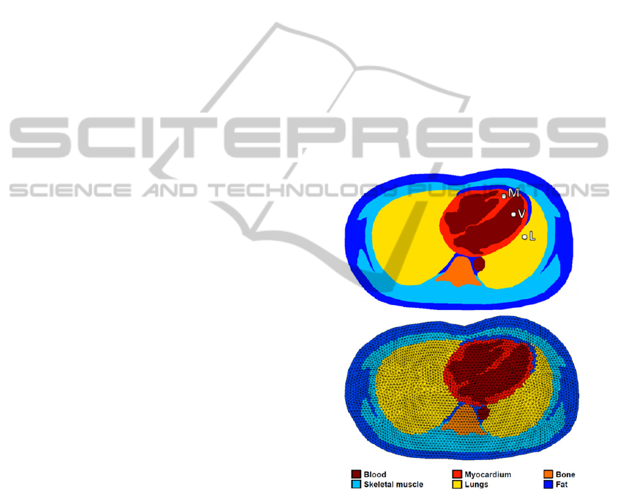
The resulting segmentation can be seen in the top

panel of Figure 1 (for one frame of the cardiac

cycle).

Figure 1: Top panel – Example of a segmented frame. The

highlighted myocardial (M), ventricular (V) and anterior

lung (L) locations will be used in Section 3. Bottom panel

– The corresponding bio-impedance mesh for EIT

simulations.

2.2.2 Model Assumptions

The following assumptions were made in the

creation of our model following today’s standard for

2D EIT:

 Electrical currents travel within the volume

scanned by the MR instrument;

UnderstandingtheGenesisofCardiacSignalsinElectricalImpedanceTomography

 Organs and tissues are isotropic (Guha, 1973);

 The reactive part of the impedance of organs and

tissues is negligible in the EIT frequency range

(Malmivuo, 1995). Similarly, magnetic effects can

be neglected at those frequencies (Holder, 2005);

 The thorax contains no internal current sources

(Holder, 2005);

 All points on the body surface in contact with an

electrode have the same potential as the electrode

and at all other surface points the electrical

potential gradient normal to the surface is zero

(Guha, 1973). Under these two boundary

conditions, the generalized Laplace’s equation

governing the domain of interest has a unique

solution (Kim, 1988).

2.2.3 Bio-impedance Mesh Generation

An extruded mesh of tetrahedral elements was

generated using NETGEN and the open source

EIDORS toolbox (Grychtol, 2012), and fits the

subject’s thorax contour in the scanned oblique

plane. At each frame of the cardiac cycle, each finite

element was assigned an electrical conductivity

value of the organ or tissue it belonged to in the time

laps of the current frame. The biological values of

electrical conductivity used in this model are listed

in Table 1.

Table 1: Tissue conductivities for an excitation frequency

of 200 kHz (Gabriel, 1996).

Tissue Conductivity (S·m

-1

)

Blood 7 × 10

-1

Skeletal muscle 4 × 10

-1

Myocardium 2.5 × 10

-1

Lungs (inflated) 8.5 × 10

-2

Bone 8.5 × 10

-2

Fat 2.5 × 10

-2

2.3 EIT Simulations

2.3.1 Simulated Scenarios

Three different 2D dynamic meshes were created,

each depicting a specific cardiac behaviour:

 Scenario A. Only the dynamics of the filling and

emptying cardiac cavities are used in this model

while the myocardium remains static throughout

the whole cardiac cycle (the same segmentation is

used for all frames, thereby suppressing other

changes). Similarly, all other organs and tissues

remain static for all frames. Therefore, this

scenario simulates blood volume-related

impedance changes only.

 Scenario B. Only the dynamics of the myocardium

is maintained in this model. The cardiac cavities

remain static throughout the whole cardiac cycle

(the same segmentation is used for all frames, thus

suppressing other changes). Similarly, all other

organs and tissues remain static for all frames.

Therefore, this scenario simulates cardiac motion-

induced impedance changes only.

 Scenario C. The dynamics of both, the cardiac

cavities and the myocardium are simulated in this

model. All other organs and tissues remain static

throughout the whole cardiac cycle. Therefore, this

scenario simulates both blood volume-related and

motion-induced impedance changes.

Modelling variations in blood volume and heart

motion separately allows isolating and thus

quantifying the effect of each one of these factors

affecting the global cardiac impedance change.

2.3.2 Image Sequences Reconstruction

EIT reconstruction is a severely ill-conditioned

inverse problem. The diffusive nature of electrical

current propagation only adds up to the complexity.

Obtaining absolute impedance values in EIT is not

only of great difficulty, but not necessary for most

EIT-based biomedical applications, which are more

interested in functional information (namely, the

variation of impedance around a reference baseline

value) (Denai, 2010). For this reason, difference EIT

is typically used. Instead of directly considering the

voltage measurements  and the conductivity

distribution , it makes use of difference data





, where 



is a reference set of voltages

typically obtained by averaging the measurements of

the first frames of an EIT recording. It corresponds

to the so-called background conductivity distribution





, used to define the difference conductivity

distribution 



. As a result, linear EIT

reconstruction can be represented by an inverse

matrix R, which translates difference measurements

 into a difference conductivity image 









(1)

The computation of the inverse matrix  depends on

the reconstruction method. In that context, the

GREIT algorithm (Adler, 2009) distinguishes itself

by encoding performance requirements directly

within the inverse matrix. In particular,  is

pretrained by optimizing several figures of merit

such as amplitude response and position error.

Evaluating how much blood volume variations

and heart motion affect – particularly in terms of

amplitude – the the global cardiac impedance signal,

BIOSIGNALS2014-InternationalConferenceonBio-inspiredSystemsandSignalProcessing

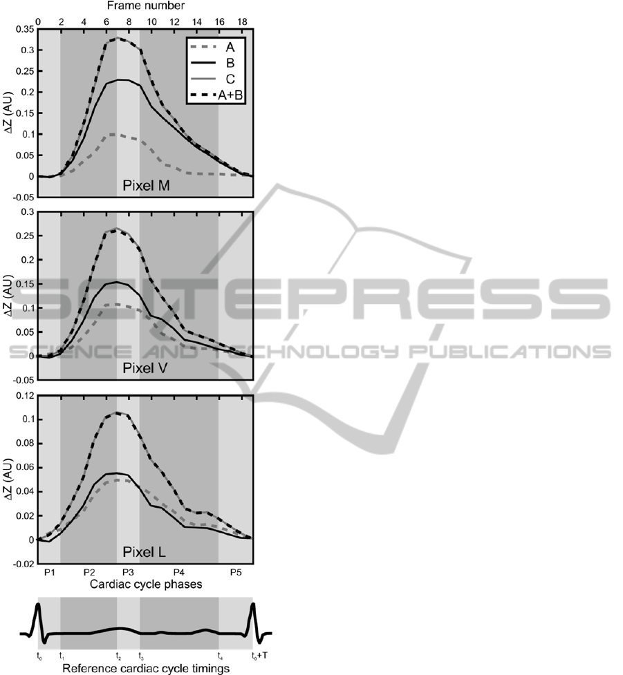
Figure 2: Impedance change occurring at the myocardial

(M), ventricular (V) and anterior lung (L) pixels for all

scenarios including the control scenario. A schematic ECG

is also displayed as an illustrative timing reference. The

meaning of the cardiac phases P1 to P5 (light and dark

grey areas) and their associated reference timings t

to t

detailed in Section 4.

requires such performance criteria to be optimal.

Consequently, the GREIT algorithm was used to

perform EIT simulations for each of the three

specific scenarios described in Section 2.3.1.

Difference data were obtained by using the first

frame (representing the end of diastole) as reference

data set. Each simulated scenario (A, B and C)

resulted in a 20-frame sequence of 60 × 40 pixel

images.

2.3.3 Control Scenario

An injected electrical current flowing through the

heart will sequentially go through tissues belonging

to the cardiac cavities and the myocardium, similarly

to a current flowing through impedances connected

in series. As a consequence, the impedances of

scenario C should theoretically be similar to the sum

of the impedances of scenarios A and B, since it

encompasses both of their respective behaviours

(blood volume-related impedance changes and

motion-induced impedance changes). For this

reason, a control scenario (scenario A+B) was

virtually created by summing the image sequences

reconstructed in scenarios A and B. It is expected to

behave similarly to scenario C.

3 RESULTS

Figure 2 illustrates, for all scenarios (A, B and C) as

well as the control scenario A+B, the impedance

changes occurring at the myocardial (M), ventricular

(V) and anterior lung (L) pixels shown in Figure 1.

Figure 3a illustrates the peak systolic impedance

value (value at frame 7) for all scenarios, including

the control scenario, at the myocardial (M),

ventricular (V) and anterior lung (L) pixels, while

Figure 3b illustrates the percentage of contribution

of blood volume-related (scenario A) and motion-

induced (scenario B) impedance changes to the

global impedance change (scenario C).

4 DISCUSSION

Three different scenarios were investigated to

evaluate the influence of blood volume changes and

heart motion on the EIT cardiac signals. A 2D

dynamic bio-impedance model was created from the

segmentation MR images. Three cardiac behaviours

– namely, blood volume-related (scenario A),

motion-induced (scenario B) or both blood volume-

related and motion-induced (scenario C) impedance

changes – were simulated, and EIT image sequences

reconstructed. A control scenario A+B was created

virtually by summing the image sequences of the

first two scenarios.

UnderstandingtheGenesisofCardiacSignalsinElectricalImpedanceTomography

In the following discussion, we first verify the

validity of the impedance waveforms observed at

three specific pixel locations (Section 4.1). We then

investigate the influence of each impedance-

affecting factor to the global cardiac EIT signal

(Section 4.2). Finally, we highlight some limitations

of our model and suggest some possible future

investigations (Section 4.3).

4.1 Impedance Waveforms

Morphology Validation

A standard cardiac cycle can be subdivided into two

isovolumetric phases (P1 and P3 in Figure 2), during

which blood volume remains constant in the

ventricles, and three anisovolumetric phases (P2, P4

and P5), during which changes in blood volume

occur.

In scenario A (dashed grey curves in Figure 2),

the only impedance-affecting factor is the change in

blood volume induced by volume variations of the

cardiac cavities. Shortly after the R peak of the ECG

(at time t

, corresponding to frame 0 in Figure 2), the

first isovolumetric phase (P1) begins. No variation

in blood volume occurs and thus the impedance

waveform remains flat. When the semilunar valves

open at t

≈ t

+ 80 ms (Levick, 2010)

(corresponding to frame 2), the first anisovolumetric

phase (ventricular ejection) starts, and blood volume

decreases in the cardiac cavities (phase P2 in Figure

2). The heart thus becomes less conductive and its

impedance increases steeply. A short isovolumetric

relaxation phase follows (P3). At t

≈ t

+ 440 ms

(Levick, 2010) (frame 9), when the atrioventricular

valves open, the ventricular volume starts returning

(rapidly at first, then slowly) to its baseline value as

ventricular filling begins (phase P4 in Figure 2). At

the start of atrial systole at t

≈ t

+ T – 160 ms

(Levick, 2010) (frame 16), where T is the cardiac

period, ventricular blood volume increases slightly

while atrial volume decreases by the same amount,

thus not influencing significantly the global

impedance change (phase P5 in Figure 2).

In scenario B (solid black curves in Figure 2),

only the dynamics of the myocardium are simulated.

The remaining organs and tissues remain static. This

scenario thus simulates motion-induced impedance

changes. During ventricular systole (phase P2 in

Figure 2), longitudinal shortening of the

myocardium begins as the apex is pulled towards the

atrioventricular plane. The space occupied by the

myocardium during diastole becomes occupied by

the pericardium, the conductivity of which is ten

times smaller than that of the cardiac muscle (Table

1). As a result, impedance increases abruptly. As the

semilunar valves close, the myocardium undergoes

elastic recoil and starts reoccupying the space it left

during ventricular systole, thus producing an

impedance decrease (phase P4 in Figure 2). The

synchrony between the waveforms of scenarios A

and B relates on the one hand to the simultaneous

beginning of the ejection phase and the myocardial

contraction, and on the other hand to the fact that the

opening of the atrioventricular valves (and thus

ventricular refilling) is caused by a sharp decrease in

pressure due to myocardial relaxation (Levick,

2010).

In scenario C (solid grey curves in Figure 2),

which aims at reflecting the real behaviour of the

heart, the dynamics of both, the cardiac cavities and

the myocardium are maintained to simulate both,

blood volume-related and motion-induced

impedance changes. The remaining organs and

tissues are static. As the strong similarity between

the solid grey and dashed back curves (scenario C

and control scenario A+B) of Figure 2 illustrates, the

contributions of blood volume variations and heart

motion add up to produce the impedance changes

observed in scenario C.

Figure 3: Left panel – Peak systolic impedance value for

all scenarios, including the control scenario, at the

myocardial (M), ventricular (V) and anterior lung (L)

pixels. Right panel – Contribution of blood volume-related

(scenario A) and motion-induced (scenario B) impedance

changes to the global impedance change (scenario C).

These percentages were computed as the ratio of the peak

systolic values of scenarios A and B (Figure 3a) with those

of scenario C.

4.2 Influence of each Factor Affecting

Impedance

The impedance changes occurring at three different

BIOSIGNALS2014-InternationalConferenceonBio-inspiredSystemsandSignalProcessing

anatomical locations (M, V and L, depicted in

Figure 1) were investigated. The resulting

impedance waveforms are shown in Figure 2. It is

worth noting that the diffusive nature of electrical

current propagation makes the mapping of function

onto anatomy challenging (i.e. a pixel identified as

belonging to a given organ or tissue using MR

information does not necessarily only reflect the

functional impedance information of the said organ

or tissue). For instance, our anterior lung pixel (L) is

expected to be slightly affected by both, cardiac

blood volume-related and motion-induced

impedance changes, because of its proximity to both

sources of perturbations. Similarly, motion-induced

impedance changes are expected to be larger in the

myocardial (M) pixel than in the ventricular (V)

pixel. The opposite is expected for blood volume-

related changes.

These assumptions are confirmed in Figure 3a,

which illustrates how the amplitude of motion-

induced impedance changes (scenario B) decreases

as one moves away from the heart’s long axis (away

from pixel M). Conversely, the amplitude of blood

volume-related impedance changes (scenario A) is

maximal when measured in the ventricular pixel (V).

The amplitude of the impedance change in the

anterior lung pixel (L) is significantly smaller for

both factors. It would be interesting in a future study

to compare this amplitude to that of impedance

changes of pulmonary origin to assess the level of

perturbation caused by cardiogenic impedance

variations on the neighbouring lung region.

Figure 3b quantifies the influence of each factor

to the cardiac EIT signal. Based on these

simulations, it appears that in the myocardial (M)

and in the ventricular (V) pixels the signal is

dominated by impedance changes originating from

the heart’s motion. In the anterior lung pixel (L) the

influence of both factors is approximately the same.

According to our model, it thus appears that the

impedance change originating from the heart’s

motion is the main factor affecting the global cardiac

impedance change.

4.3 Limitations

Our observations have provided novel insights into

the understanding of the genesis of cardiac

impedance changes in EIT. However, these results

necessitate further investigations, as they are based

on a simplified simulation model showing three

main limitations:

 The model is two-dimensional, while electrical

currents are known to propagate in three

dimensions. Impedance changes occurring above

and below the electrode plane are thus not

considered adequately.

 The blood volume variations and the motion of the

remaining organs and tissues are not modelled. In

particular, the influence of respiratory movements,

pulmonary perfusion and blood volume changes in

the major elastic arteries, is not taken into account.

While this allows isolating the influence of each

individual factor in simulations, it neglects their

interdependencies acting in reality.

 Only one subject was used in our experiment.

5 CONCLUSIONS

We developed a 2D dynamic bio-impedance model

for EIT simulations. Our study shows that EIT

signals in the heart area might be dominated by

motion-induced impedance changes.

Based on these important observations, it would

be interesting to investigate possible solutions, such

as exploiting larger frequency content or a multi-

frequency approach to perform source separation, or

enhancing the EIT signals using motion-

compensating models. It is worth mentioning that

these approaches could be exploited either before or

after image reconstruction.

Additionally, experimental and clinical studies

should be performed to confirm what we observed in

our model.

ACKNOWLEDGEMENTS

This work was made possible by grants from the

SNSF/Nano-Tera.CH’s project OBESENSE

(20NA21-1430801).

REFERENCES

Adler, A., Arnold, J. H., Bayford, R. et al., 2009. GREIT:

a unified approach to 2D linear EIT reconstruction of

lung images, Physiological Measurement, vol. 30, no.

16, pp. S35–S55.

Barber, D. C., 1990. Quantification in impedance imaging,

Clinical Physics and Physiological Measurement, vol.

11 (suppl A), pp. 45-56.

Bayford, R. H., 2006. Bioimpedance tomography

(electrical impedance tomography), Annual Review of

Biomedical Engineering, vol. 8, pp. 63-91.

Borges, J. B., Suarez-Sipmann, F., Böhm S. H. et al.,

2011. Regional lung perfusion estimated by electrical

UnderstandingtheGenesisofCardiacSignalsinElectricalImpedanceTomography

impedance tomography in a piglet model of lung

collapse, Journal of Applied Physiology, vol. 112, no.

11, pp. 225-236.

Braun, F., 2013. Systolic Time Intervals Measured by

Electrical Impedance Tomography (EIT), Swiss

Federal Institute of Technology, Zurich, Switzerland.

DOI: http://dx.doi.org/10.3929/ethz-a-009947722.

Brown, B.H., Leathard, A., Sinton, A. et al., 1992. Blood

flow imaging using electrical impedance tomography,

Clinical Physics and Physiological Measurement, vol.

13 (suppl A), pp. 175-179.

Deibele, J. M., Luepschen H. and S. Leonhardt, 2008.

Dynamic separation of pulmonary and cardiac

changes in electrical impedance tomography,

Physiological Measurement, vol. 29, no. 16, pp. S1-

S14.

Denai, M. A., Mahfouf, M., Mohamad-Samuri, S. et al.,

2010. Absolute Electrical Impedance Tomography

(aEIT) Guided Ventilation Therapy in Critical Care

Patients: Simulations and Future Trends, IEEE

Transactions on Information Technology in

Biomedicine, vol. 14, no. 13, pp. 641-649.

Fagerberg, A., Stenqvist, O. and Åneman, A., 2009.

Monitoring pulmonary perfusion by electrical

impedance tomography: an evaluation in a pig model,

Acta Anaesthesiologica Scandinavica, vol. 53, no. 12,

pp. 152-158.

Ferrario, D., Grychtol, B., Solà, J. et al., 2012. Towards

morphological thoracic EIT: Major signal sources

correspond to respective organ locations in CT, IEEE

Transactions on Biomedical Engineering, vol. 59, no.

111, pp. 3000-3008.

Frerichs, I., Hinz, J., Herrmann, P. et al., 2002. Regional

lung perfusion as determined by electrical impedance

tomography in comparison with electron beam CT

imaging, IEEE Transactions on Medical Imaging, vol.

21, no. 16, pp. 646-652.

Frerichs, I., Pulletz, S., Elke, G. et al., 2009. Assessment of

changes in distribution of lung perfusion by electrical

impedance tomography, Respiration, vol. 77, no. 13,

pp. 282-291.

Gabriel, S., Lau, R. W. and Gabriel, C., 1996. The

dielectric properties of biological tissues: III.

Parametric models for the dielectric spectrum of

tissues, Physics in Medicine and Biology, vol. 41, no.

111, pp. 2271–2293.

Grant, C. A., Pham, T., Hough, J. et al., 2011.

Measurement of ventilation and cardiac related

impedance changes with electrical impedance

tomography, Critical Care, vol. 15, no. 11, p. R37.

Grychtol, B., Lionheart, W. R. B., Bodenstein, M. et al.,

2012. Impact of Model Shape Mismatch on

Reconstruction Quality in Electrical Impedance

Tomography, IEEE Transactions on Medical Imaging,

vol. 31, no. 19, pp. 1754-1760.

Guha, S. K., Khan, M. R. and Tandon, S. N., 1973.

Electrical field distribution in the human body,

Physics in Medicine and Biology, vol. 18, no. 5, pp.

712-720.

Hellige, G., Hahn, G., 2011.

Cardiac-related impedance

changes obtained by electrical impedance

tomography: an acceptable parameter for assessment

of pulmonary perfusion?, Critical Care, vol. 15, p.

430.

Holder, D. S., 2005. Electrical impedance tomography:

methods, history and applications, Institute of Physics

Publishing. London.

Kim, D. W., Baker, L. E., Pearce, J. A. and Kim, W. K.,

1988. Origins of the impedance change in impedance

cardiography by a three-dimensional finite element

model, IEEE Transactions on Biomedical Engineering,

vol. 35, no. 112, pp. 993-1000.

Kunst, P. W. A., Vonk-Noordegraaf, A., Hoekstra, O. S. et

al., 1998. Ventilation and perfusion imaging by

electrical impedance tomography: a comparison with

radionuclide scanning, Physiological Measurement,

vol. 19, no. 14, pp. 481–490.

Leathard, A. D., Brown, B. H., Campbell, J. et al., 1994. A

comparison of ventilatory and cardiac related changes

in EIT images of normal human lungs and of lungs

with pulmonary emboli, Physiological Measurement,

vol. 15 (suppl 2A), pp. A137-A146.

Levick, J. R., 2010. An introduction to cardiovascular

physiology, Arnold. London, 5

edition.

Malmivuo, J. and Plonsey, R., 1995. 7: Volume source

and volume conductor, in Bioelectromagnetism:

Principles and Applications of Bioelectric and

Biomagnetic Fields, University Press. New York.

McArdle, F. J., Suggett, A. J., Brown, B. H. and Barber,

D. C., 1988. An assessment of dynamic images by

applied potential tomography for monitoring

pulmonary perfusion, Clinical Physics and

Physiological Measurement, vol. 9 (suppl A), pp. 87-

91.

Nguyen, D. T., Jin, C., Thiagalingam, A. and McEwan, A.

L., 2012. A review on electrical impedance

tomography for pulmonary perfusion imaging,

Physiological Measurement, vol. 33, no. 5, pp. 695–

706.

Smit, H. J., Vonk-Noordegraaf, A., Marcus, J. T. et al.,

2004. Determinants of pulmonary perfusion measured

by electrical impedance tomography, European

Journal of Applied Physiology, vol. 92, no. 1, pp. 45-

49.

Vonk-Noordegraaf, A., Kunst, P. W. A., Janse, A. et al.,

1998. Pulmonary perfusion measured by means of

electrical impedance tomography, Physiological

Measurement, vol. 19, no. 12, pp. 263–273.

Vonk-Noordegraaf, A., Janse, A., Marcus, J. T. et al.,

2000. Determination of stroke volume by means of

electrical impedance tomography, Physiological

Measurement, vol. 21, no. 12, pp. 285–293.

BIOSIGNALS2014-InternationalConferenceonBio-inspiredSystemsandSignalProcessing