Learning with Kernel Random Field and Linear SVM

Haruhisa Takahashi

The University of Electro-Communications, Choufushi Tokyo 182-8585, Japan

Keywords:

Autocorrelation Kernel, MRF, Mean-ﬁeld, Fisher Score, Deep Learning, SVM.

Abstract:

Deep learning methods, which include feature extraction in the training process, are achieving success in

pattern recognition and machine learning ﬁelds but require huge parameter setting, and need the selection

from various methods. On the contrary, Support Vector Machines (SVMs) have been popularly used in these

ﬁelds in light of the simple algorithm and solid reasons based on the learning theory. However, it is difﬁcult

to improve recognition performance in SVMs beyond a certain level of capacity, in that higher dimensional

feature space can only assure the linear separability of data as opposed to separation of the data manifolds

themselves. We propose a new framework of kernel machine that generates essentially linearly separable

kernel features. Our method utilizes pretraining process based on a kernel generative model and the mean

ﬁeld Fisher score with a higher-order autocorrelation kernel. Thus derived features are to be separated by

a liner SVM, which exhibits far better generalization performance than any kernel-based SVMs. We show

the experiments on the face detection using the appearance based approach, and that our method can attain

comparable results with the state-of-the-art face detection methods based on AdaBoost, SURF, and cascade

despite of smaller data size and no preprocessing.

1 INTRODUCTION

A deep architecture is a recent trend in classiﬁcation

problems to obtain ﬁnally ﬂexible linearly separable

features against previous trend depending on rich de-

scriptors such as SIFT, HOG, or SURF (Bengio et.al.

2012). The linear separability of data is a milestone

for a good feature representation, and is realized by

a higher dimensional kernel feature space in SVM as

well as stacked layered representation in neural net-

works.

However, linear separability of training examples

can not necessarily result in a good generalization

if the feature extractor is not ﬁtted in the probabil-

ity distribution of instances. For example, in SVMs,

kernels are required to reﬂect on the distribution of

instances for better generalization, and yet they are

hard to come by. Fisher kernel (Jaakkola & Haussler

1998) is an exceptional example, in that it is based

on a generative model, but not popularly used due

to its computational cost and speciality. There are

other researches to combine the generative models

with kernels but they take in similar problems (Laf-

ferty Zhu & Liu 2004),(Lafferty McCallum & Pereira

2004),(Roscher 2010).

Although SVM is a general-purpose nonlinear

classiﬁer where its kernel feature space can linearly

separate training data, the data manifolds themselves

are not necessarily separated each other. This is a rea-

son why the deep learning often outperforms SVM in

classiﬁcation capacity. In this observation we aim at a

feature extractor based on data distribution, which can

give linearly separable data manifolds to be combined

with linear SVM classiﬁer.

We directly use Fisher score of Markov random

ﬁeld (MRF) as a feature extractor that can give es-

sentially linearly separable representation of the prob-

lem. In order to represent data manifolds effectively

we need to transform MRF into a kernel based repre-

sentation. Fortunately, the cliques in MRF are units of

computing higher order autocorrelation, from which

we can reach a deﬁnition of a novel autocorrelation

kernel and the concept of kernel random ﬁelds (KRF).

In this context Fisher score can be represented as a

simple form in terms of the autocorrelation kernels

and their differences with the mean value of KRF. Fi-

nally we propose a SVM-like classiier deﬁned by a

linear SVM applied on this feature.

We propose an efﬁcient algorithm to compute the

autocorrelation kernel in the linear order for the in-

put length. KRF is computed by using the variational

mean ﬁeld that leads the Fisher score to a simple ker-

167

Takahashi H..

Learning with Kernel Random Field and Linear SVM.

DOI: 10.5220/0004792601670174

In Proceedings of the 3rd International Conference on Pattern Recognition Applications and Methods (ICPRAM-2014), pages 167-174

ISBN: 978-989-758-018-5

 2014 SCITEPRESS (Science and Technology Publications, Lda.)

nel difference. We show with computer experiments

on the face discrimination problem that our model

performs better than SVM, and can give comparable

results with speciﬁcally tuned face detectors, despite

the smaller training data size.

2 OUTLINE OF THE MODEL

Data manifolds tend to be ﬂexibly linearly separated

by a deep architecture, while indeed data represen-

tation in SVM or multilayer neural networks are lin-

early separated, but data manifolds are not necessar-

ily separated. In order to obtain a linearly separa-

ble representation, the feature extractor should be de-

signed so as to have a potential that takes smaller

values for the object class instances than for the out-

of-class instances. For example, in Auto-Encoder or

Sparse Coding, difference between the input vectors

and the reconstructed vectors is designed to be min-

imum, thus becomes a potential on the data. In a

deep architecture, such feature extractors are stacked,

and enabling to regularize the potential (Erhan et.al.

2010), making the data manifolds be linearly sepa-

rated.

Another idea to obtain a regularized feature poten-

tial comes from the generative models. Fisher kernel

is the one that reﬂects this idea, and deﬁned by the

inner product of Fisher score, although a problem of

computational efﬁciency is involved. Given a model

P(x|θ) Fisher score is deﬁned by

(x) =

∂logP(x|θ)

∂θ

(1)

The vector score of Eq.(1) takes a value near 0 for an

input vector x of the class, if the parameter θ is prop-

erly trained as a model of the class. This implies that

Fisher kernel is an over-transformed representation in

the sense that kernel values of x

near 0 does not

necessarily mean both x

and x

belong to the class.

In this reason we propose a method to directly utilize

Fisher score with MRF unlike Fisher kernel method

such as (Jaakkola & Haussler 1998).

MRF models objects with auto-correlative units

called cliques, and have been applied for wide range

of signal processing or pattern analysis ﬁelds. If we

adopt MRF as a basic generative model for calculat-

ing Fisher score, we must have suffer from combi-

natorially huge number of model parameters corre-

sponding to the number of cliques.

A compact expression of features can be obtained

from the kernel representation of the random ﬁeld. In

order to take the autocorrelations of cliques into ker-

nels, we will deﬁne a feature vector consist of cliques

in section 3, and the kernel is deﬁned by the inner

product of feature vectors. Note that our deﬁnition of

autocorrelation kernel does not include the second or

a higher order of single variables. This reduces the

computational complexity of the kernel to linear or-

der.

The higher autocorrelation kernel introduced in

section 3 is able to reﬂect a difference of higher order

autocorrelations, while the popular Gaussian or poly-

nomial kernel depends only on the difference of input

vector values. A higher order autocorrelation kernel

was examined in (Horikawa 2004), in which direct

inner product of feature vectors of higher order auto-

correlations was used, besides higher order moments

of single variables were used in his setting. Thus it

requires huge computational efforts.

If we use our deﬁnition of higher autocorrelation

kernel, we can deﬁne Kernel Random Field (KRF) for

n dimensional discrete states x as follwos:

P(x|µ) =

exp

−

∑

ℓ=1

ℓ

K(ξ

ℓ

,x)

(2)

which is equivalent to MRF, where Z is the parti-

tion function, ξ

ℓ

are m training examples, and µ

ℓ

are

the model parameters. For the practical situations,

computation of KRF of eq.(2) is hard for seeking Z.

We apply the mean ﬁeld approximation to derive the

mean ﬁeld Fisher score expression in section 5:

ℓ

′

(ξ

ℓ

) = K(ξ

ℓ

′

,ξ

ℓ

) − K(ξ

ℓ

′

, ¯x) (3)

where ¯x,ξ

ℓ

′

,ξ

ℓ

are the mean of the states in the mean

ﬁeld, ℓ

′

th in-class training instance, and ℓth training

instance, respectively. In fact, on one hand, for the in-

class instances ξ

ℓ

the ﬁrst and the second terms in the

right hand side of eq.(3) take similar (comparatively

large) values, and the subtraction results in near 0. On

the other hand, if ξ

ℓ

is an outside-the-class instance,

the ﬁrst term of the right hand side of eq.(3) takes a

small value, and the subtraction results in negatively

large. As the result, the features of eq.(3) becomes lin-

early separable, because the problem is reduced to the

majority voting with the negativelycontinuous values.

We propose a learning scheme using a linear SVM

to discriminate the Fisher score features given in

eq.(3). Then the training process is divided in two

steps; in the ﬁrst step the mean ﬁeld KRF is trained for

the class data, and in the second step, the linear SVM

is trained on features of eq.(3) using the all training

data. We will show computer experiments on the face

detection problem in section 6, and show that the pro-

posed scheme works well to get far better results than

SVMs. The results are comparable to a state-of-the-

art face detection system using SURF, cascade, and

AdaBoost (Li & Zhang 2013).

ICPRAM2014-InternationalConferenceonPatternRecognitionApplicationsandMethods

168

3 HIGHER AUTOCORRELATION

KERNEL

The autocorrelation kernel previously used one

(Horikawa 2004) was simply computed by an inner

product of feature vectors. The dimension of the fea-

ture vectors is O(n

) according to an input vector

size n and a ﬁxed order of autocorrelation d ≪ n. In

our deﬁnition of higher autocorrelation kernel, we ex-

cluded the second or a higher moment of single vari-

ables from the feature vectors. In light of this we can

compute the higher autocorrelation kernel in O(n) for

ﬁxed d ≪ n, which is shown below.

Let an input vector be x = (x

,...,x

)

. Then we

deﬁne a higher autocorrelation feature vector up to

dth order as

φ(x) = (1;x

,...x

,...,x

n−1

;...;

...,x

n−d+1

· · · x

)

(4)

where the general term representing dth autocorre-

lation is x

· · · x

,(i

< i

,...,< i

). Then the

higher autocorrelation kernel is deﬁned by K(x, z) =

φ(x)

· φ(z). We will show an efﬁcient computational

algorithm of K(x,z) in the followings.

3.1 Expression with Symmetric

Polynomial

The higher autocorrelation kernel can be represented

using the symmetric polynomial given by

(x) = 1

(x) = x

+ ... + x

(x) = x

+ x

+ ... + x

n−1

(x) = x

+ x

+ ... + x

n−2

n−1

· · · · · · · · ·

Let y

= x

. Then

K(x,z) =

∑

i=0

(y), y = (y

,...,y

)

(5)

If degree of the kernel should be speciﬁed, it would be

written as K

(x,z). Notice that the general dth degree

polynomial kernel (< x,z > +c)

takes O(n), but the

direct computation of eq.(5) takes O(n

),d ≪ n pro-

portional to the number of monomials.

3.2 Computational Algorithm of O(n)

We show the next lemma reducing the computation of

eq.(5) to a recursive formula.

Lemma 1. Let d ≤ n be ﬁxed. Then S

is computed

from S

,(d/2 ≥ k) in O(n) as

n−[d/2]

∑

i=[d/2]

−

i−1

[d/2]

−

[d/2]

where [·]

−

, [·]

represent the ﬂoor and the ceil inte-

gers, respectively, and

i+1

− x

i+1

k−1

(i = n− 1,...,k),

= S

= x

∑

j=i+1

k−1

(proof) First we show the computational complexity.

Sum of

i−1

[d/2]

−

and S

[d/2]

is O(n). For ﬁxed k, both of

and S

is computed in O(n). The number of recur-

sive iteration to compute these factors is less than or

equal to log

d. Thus totally the computational com-

plexity is O(n). In order to show formally the recur-

sive formulae in the lemma, we can use the induction.

However, as it makes too much complicated, we sat-

isﬁed with exemplifying d = 1,...,4 in the following.

Q.E.D.

Example S

: Note that S

= x

, (i = 1, ..., n), thus

∑

i=1

. Then

becomes the ﬁrst degree sym-

metric polynomial of x

,...,x

, and

i+1

− x

i+1

, (i = n− 1,...,1),

= x

+ ... + x

Thus

= S

: S

is computed using S

∑

i=2

i−1

Now S

is the sum of terms containing both x

and

, (i < j) simultaneously in S

. Thus

= x

∑

j=i+1

= x

i+1

+ .. + x

), (i = 1,...,n− 1),

Then

is deﬁned as the second degree symmetric

polynomial of x

,...,x

, and determined by

i+1

− x

i+1

(i = n− 1,...,2),

= S

and S

: Since S

is sum of the product of S

)

and

i−1

(

i−1

) for all i,

n−1

∑

i=2

i−1

n−1

∑

i=2

i+1

Now S

is sum of terms containing both x

and x

, (i <

j) simultaneously in S

. Thus

= x

∑

j=i+1

LearningwithKernelRandomFieldandLinearSVM

169

0 500 1000 1500 2000

0.05

0.1

0.15

0.2

0.25

0.3

0.35

vector size

d=4

d=2

Figure 1: Computational time of higher autocorrelation ker-

nels for size n input vectors.

Further,

is deﬁned as the third degree symmetric

polynomial of x

,...,x

, and determined by

i+1

− x

i+1

(i = n− 1,...,3),

= S

Similarly we can ﬁnd

n−2

∑

i=2

i−1

∑

i=4

i−1

n−1

∑

i=3

i−1

and

i+1

− x

i+1

(i = n− 1,...,4),

= S

= x

∑

j=i+1

In general we need [k/2]

th degree S

for seeking

kth degree symmetric polynomial.

Figure 1 shows computational time of autocorrela-

tion kernels for vectors of size n, which are randomly

generated. We can conﬁrm O(n) from this experi-

ment. It is important in applying the autocorrelation

kernel that either the input vectors should be normal-

ized with norms or the kernels are normalized as

K(x,z) =

K(x,z)

K(x,x)K(z,z)

Autocorrelation kernel must be advantageous for

pattern discrimination tasks. We compared the auto-

correlation kernel with the polynomial kernel using

SVM classiﬁer for real data of face detection. We ran-

domly chose 2000 face data and 2000 non-face data

from training data of CMU+MIT dataset (see section

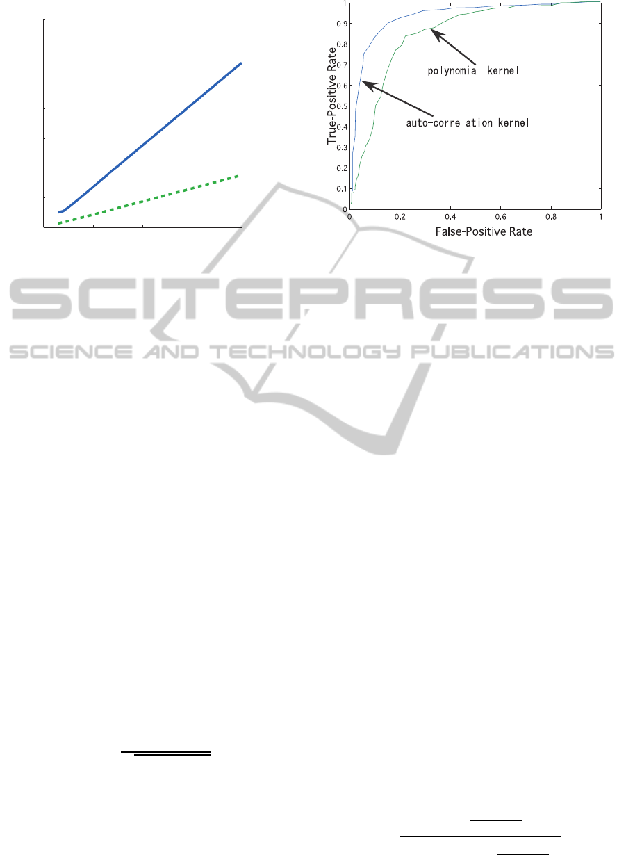
Figure 2: ROC curves of normalized autocorrelation and

polynomial kernels (7th degree) with SVM.

6). We leave out 400 face and non-face data from

them, and remaining 1600 data for each class are used

for training. Figure 2 compares the ROC curves for

7th degree normalized autocorrelation and polyno-

mial kernels. The autocorrelation kernel shows much

better discrimination performance than the polyno-

mial kernel. The discrimination performance of (nor-

malized) polynomial kernel is same or similar for the

degree greater than or equal to 3.

4 MEAN FIELD KRF

In this section we introduce computationally feasible

feature extraction based on MRF.

4.1 Variational Mean Field of KRF

We derive a variational mean ﬁeld expression of KRF.

Let the logarithmic potential function of KRF of

eq.(2) be

(x) = −

∑

ℓ=1

ℓ

K(ξ

ℓ

,x), (6)

and let states x

take values k ∈ {0, 1, 2,...,r− 1}. Let

Q(x|µ) =

∏

i=1

be the mean ﬁeld probability func-

tion, in which q

= 1−

∑

r−1

k=1

, and r

= P(x

= k|µ)

be the marginal probability function for KRF given by

P(x|µ). Then the following lemma holds.

Lemma 2. Let E

(x)} be the mean of V

(x) with

respect to P(x|µ). Then Q(x|µ) satisﬁes

exp



−

∂E

(x)}

∂q



∑

r−1

′

exp



−

∂E

(x)}

∂q

′



ICPRAM2014-InternationalConferenceonPatternRecognitionApplicationsandMethods

170

(proof) Mean ﬁeld probability Q is derived minimiz-

ing the following KL divergence

KL(P,Q) =

∑

P(x|µ)ln

P(x|µ)

= −

∑

i=1

r−1

∑

k=1

lnq

− E

(x)} − lnZ (7)

Taking the partial derivative of the right hand side in

the second equality of eq.(7) w.r.t. q

, and putting 0,

we can ﬁnd that r

= q

. Placing this relation back

into eq.(7), and taking the partial derivative q.r.t. q

put 0, the resulting equation gives the lemma.

Q.E.D.

Now let the mean of V

(x) on Q(·|µ) be

(x)}. We will use an approximation that the

partial derivative of E

(x)} w.r.t. q

is replaced

by the partial derivative of E

(x)} w.r.t. q

4.2 Mean Field Potential

We take advantage of the d linearity of the autocorre-

lation kernels to derive mean ﬁeld potential of KRF.

Lemma 3. Let the expression ¯· represent the mean by

the marginal probability function

∏

i=1

. Then

K(ξ

ℓ

,x) = K(ξ

ℓ

, ¯x)

K(ξ

ℓ

(i)

[k]) = K(ξ

ℓ

, ¯x

(i)

[k])

where the following notation is used

(i)

[y] = (z

,...,z

i−1

,y,z

i+1

,...,z

)

(proof) From colinearity of the inner product

K(ξ

ℓ

,x) = < φ(ξ

ℓ

),φ(x) >

Taking the mean w.r.t. each entry x

·· · x

of the vec-

tor φ(x),

· · · x

= ¯x

· · · ¯x

, (i

< ... < i

)

and the lemma is proved. Q.E.D.

Lemma 4. For µ = o(µ)

∂r

∂µ

ℓ

′

= r



K(ξ

ℓ

′

, ¯x

(i)

[k]) − K(ξ

ℓ

′

, ¯x)



(proof) The marginal probability is given by

∑

(i)

[k]

P(x|µ) =

∑

(i)

[k]

exp(

∑

ℓ=1

ℓ

K(ξ

ℓ

,x))

For µ = 0 KRF becomes the independent ﬁeld from

eq.(2). Thus P(x|µ) →

∏

i=1

for µ = o(µ). Using

Lemma 3

∂r

∂µ

ℓ

′

∑

(i)

[k]

K(ξ

ℓ

′

,x)P(x|µ)

−

∑

(i)

[k]

P(x|µ)

∑

K(ξ

ℓ

′

,x)P(x|µ)

∑

(i)

[k]

K(ξ

ℓ

′

,x)P(x|µ) − r

K(ξ

ℓ

′

,x)

= r



K(ξ

ℓ

′

, ¯x

(i)

[k]) − K(ξ

ℓ

′

, ¯x)



Q.E.D.

Lemma 5. For µ = o(µ)

∂E

(x)}

∂µ

ℓ



o(µ)

∂E

(x)}

∂µ

ℓ



o(µ)

= −K

(ξ

ℓ

, ¯x)

where E

is the mean by the marginal

∏

i=1

(proof) Since P(x|µ) →

∏

i=1

for µ = o(µ), the ﬁrst

equality holds in the lemma. From Lemma4

∂r

∂µ

ℓ

con-

verges when µ → 0. Thus

∂E

(x)}

∂µ

ℓ

= −K

(ξ

ℓ

, ¯x)

−

∑

i=1

∑

ℓ=1

∑

ℓ

(ξ

ℓ

,x)r

...

∂r

∂µ

ℓ

...r

= −K

(ξ

ℓ

, ¯x) + o(µ)

Q.E.D.

From Lemma 5, if we take the ﬁrst term of

Maclaurin expansion w.r.t. µ

(x)} = −

∑

ℓ=1

K(ξ

ℓ

, ¯x)µ

ℓ

(8)

We denote the vector that is constructed by removing

ith entry from a vector z as

(i)

= (z

,...,z

i−1

i+1

,...,z

)

Then

∂K

(ξ

ℓ

, ¯x)

∂r

= kξ

ℓ

d−1

(ξ

(i)

ℓ

, ¯x

(i)

) (9)

where ξ

ℓ

is the ith entry of ξ

ℓ

. From Lemma 2, lemma

3, and Lemma 5, we obtain the mean ﬁeld equation

exp



∑

ℓ=1

kξ

ℓ

d−1

(ξ

( j)

ℓ

, ¯x

( j)

)µ

ℓ



∑

r−1

′

exp



∑

ℓ=1

′

( j)

ℓ

d−1

(ξ

( j)

ℓ

, ¯x

( j)

)µ

ℓ



(10)

LearningwithKernelRandomFieldandLinearSVM

171

The iterative method can applied to eq.(10) based on a

numerical analysis of the differential equation that has

an equilibrium as eq.(10). For computing eq.(10), the

evaluation of (d − 1)th degree kernel will be needed,

and when n is large this takes huge computational ef-

forts. However, if we notice that the kernels in eq.(10)

should be evaluated by vectors of z

(i)

type variables,

the essential computational time reduces to comput-

ing one kernel of K

d−1

(ξ

ℓ

, ¯x). The method is shown

in the Appendix.

5 FEATURES WITH KRF

KRF is trained by one class data, and can be applied

as a feature extractor. In this section we derive the

mean ﬁeld expression of the maximum likelihood es-

timation and Fisher score as a feature extractor.

5.1 Maximum Likelihood Estimation

Given training data {ξ

,...,ξ

}, we seek the parame-

ter that maximize the empirical log likelihood

L(µ) =

∑

ℓ=1

logP(ξ

ℓ

|µ)

If we apply the mean ﬁeld Q(x|µ) instead of KRF

P(x|µ),

∂L(µ)

∂µ

ℓ

′

∑

ℓ=1



−

∂V

(ξ

ℓ

)

∂µ

ℓ

′

∑

∂V

(x)

∂µ

ℓ

′

P(x|µ)



∑

ℓ=1



K(ξ

ℓ

′

,ξ

ℓ

) −

∑

K(ξ

ℓ

′

,x)Q(x|µ)



∑

ℓ=1



K(ξ

ℓ

′

,ξ

ℓ

) − K(ξ

ℓ

′

, ¯x)



(11)

where ℓ

′

= 1,...,k, k being the number of kernels used

in KRF. As is shown in section 4, eq. (11) holds for a

small µ. We can perform the steepest ascent method

using eq.(11) for the optimum µ.

5.2 Mean Field Fisher Score

We use the mean ﬁeld KRF as a feature extractor.

Since the log likelihood of properly trained KRF is

maximized, the Fisher (vector) score given by eq.(11)

is small for a class vector ξ

ℓ

, and large for an outside-

the-class vector. Speciﬁcally, we choose {ξ

,...,ξ

}

for k ≤ m as the kernel data, that is, for ℓ

′

= 1,...,k

∂logP

(ξ

ℓ

)

∂µ

ℓ

′

= K(ξ

ℓ

′

,ξ

ℓ

) − K(ξ

ℓ

′

, ¯x) (12)

are the k dimensional feature of each ξ

ℓ

, where ¯x is

the mean of states with Q(x|µ). As was explained in

section 2, this feature is essentially linearly separable.

In general, the number of kernels k in KRF can be

determined so as to let the training data of size m be

mostly linearly separable. In practice this holds even

for not so large k, but as will be shown in section 6,

such a k is not necessarily resulted in the best gen-

eralization even if m training data are mostly linearly

separated. We can use a linear SVM to discriminate

one class from others on features of eq.(12).

6 EXPERIMENTS

Face detection is a practically important, typical and

difﬁcult pattern recognition problem. This problem

has been studied in a quite large number of references

so far, and is appropriate to evaluate the classiﬁca-

tion power. In this section we empirically evaluate

our method using eq.(12) as a feature extractor for

the face discrimination problem. In the face discrim-

ination problem, a dataset of faces and non-faces are

cropped and resampled from original images, so that

the problem is basically equivalent to the face detec-

tion.

The face detection has been intensively studied

since the break-throughof Viola-Jones (Viola & Jones

2004), and improved using such as SURF, AdaBoost,

and Cascade (Li & Zhang 2013). Datasets of face

detection has also been renewed, and it is difﬁcult to

compare the generalization power with previous stud-

ies.

We describe the experimental results on a subset

of CMU+MIT dataset, which is out-of-date now, but

the detector of Viola-Jones was tested on this dataset.

Alvira and Rifkin (Alvira & Rifkin 2001) prepared a

subset of CMU+MIT dataset for the purpose of clas-

siﬁer evaluation, and conducted experiments of face

discrimination. We utilize their dataset for training

and testing of our classiﬁer.

In their data set each face or non-face image is

cropped to a 19 × 19 window, and each pixel has

256 grayscale values. There are 2429 face and 4548

non-face cropped images for training, and 472 face

and 23573 non-face cropped images for testing. This

dataset was previously available on the CBCL web-

page, but it is unavailable now.

For training the classiﬁer we used 2429 face im-

ages, and equipped three non-face datasets; the ﬁrst

set consists of the ﬁrst 2429 non-face images, the sec-

ond set consists of 4215 non-face images, and the

third set is constructed by adding the mirror images

of the ﬁrst set to the second set resulted in 6644 non-

face images. For testing we used 470 face images out

of 472 images (the ﬁrst one and the last one is re-

ICPRAM2014-InternationalConferenceonPatternRecognitionApplicationsandMethods

172

0 0.05 0.1 0.15 0.2 0.25 0.3 0.35

0.5

0.55

0.6

0.65

0.7

0.75

0.8

0.85

0.9

0.95

False positive rate

True positive rate

2429

4215

6644

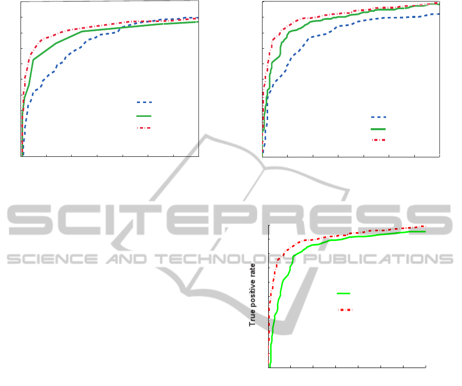
Figure 3: ROC curves for 8 training iteration of KRF corre-

sponding to non-face datasets 2429, 4215, and 6644.

moved), and randomly chosen 470 non-face images

from 23573 images.

Our approach is appearance-based, that is, the

grayscale intensity of image pixels serve as the fea-

ture. Each image is transformed into the projec-

tive space in order to normalize with intensity ratio.

Speciﬁcally, each pixel value is divided by the norm

of the image, and multiplied by 19/2, mapping almost

all pixel values into [0,1]. For discrete states of KRF

model, we discretize the pixel values in 9 values from

0 to 1 at intervals of 0.125.

We constructed KRF by 1200 autocorrelation ker-

nels with the ﬁrst 1200 training face data. The or-

der of autocorrelation is set at d = 4. Then KRF was

trained using 1600 training face data (400 data was

added to the 1200 kernel data) until the absolute value

of eq.(11) became less than 1/100 of the initial values.

We trained a linear SVMon the features of eq.(12)

using 2429 face data and each of the above described

three non-face dataset. LSVM (Mangasarian & Mu-

sicant 2001) is used for this purpose. The soft-margin

parameter of LSVM is set to 0.3∼0.5 so as to discrim-

inate almost all training data.

We show the ROC curves in Figure 3 for 8 iter-

ations and Figure 4 for 10 iterations of KRF train-

ing. In order to investigate the effectiveness of the

feature extractor with KRF (eq.(12) for 10 training

iterations), we compare it with auto-correlation ker-

nel+LSVM in Figure 5. In this ﬁgure ROC curves

are shown using 1200 kernels for KRF, and 2429

face + 6644 non-face kernels for auto-correlation ker-

nel+LSVM classiﬁer.

From these results we see that the feature rep-

resentation of KRF is essentially linearly separable.

The recent tendency of face detection is based on the

set of simple visual features called ’integral features’

0 0.05 0.1 0.15 0.2 0.25 0.3 0.35

0.5

0.55

0.6

0.65

0.7

0.75

0.8

0.85

0.9

0.95

False positive rate

True positive rate

2429

4215

6644

Figure 4: ROC curves for 10 training iteration of KRF cor-

responding to non-face datasets 2429, 4215, and 6644.

0 0.05 0.1 0.15 0.2 0.25 0.3 0.35

0.5

0.55

0.6

0.65

0.7

0.75

0.8

0.85

0.9

0.95

KRF+LSVM

Auto-Correlation kernel

False positive rate

Figure 5: ROC curves for KRF+LSVM classiﬁer with 1200

(face) kernels and auto-correlation kernel + LSVM classi-

ﬁer with 2429 face + 6644 non-face kernels.

proposed in (Viola & Jones 2004), choosing critical

visual features with AdaBoost, and cascade alloca-

tion of discriminators. The cascade allocation aims

at cut-down of detection time with discarding clearly

non-face examples at the early stage of detection.

Unfortunately results with state-of-the-art meth-

ods are not available for comparison as they are based

on a rich training data. However, as in (Li & Zhang

2013) CMU+MIT full test set is used for evaluation of

a state-of-the-art methods, and ROC curves compar-

ing with (Viola & Jones 2004) are presented, we pick

up the coresponding values from the ROC curves to

show comparison in Table 1 only for reference. From

Table 1 we can see that our classiﬁer is comparable

with the state-of-the-art detectors specialized to the

face detection.

LearningwithKernelRandomFieldandLinearSVM

173

Table 1: Recognition/detection rates(%) for false positives

(10, 20%) on CMU+MIT test set.

Systems \ False positives 10 % 20%

KRF(10 iters)+LSVM on the subset

of CMU+MIT test set

94.8 97.2

Viola & Jones 2004 92.1 93.2

SURF cascade, J.Li and Y. Zhang

(picked up from ROC curves of (Li

& Zhang 2013))

(94

) –

1 Corresponding point to 92% value of Viola & Jones

7 CONCLUSIONS

In this paper we proposed a new kernel machine

called KRF+LSVM, and showed that its classiﬁcation

capability out performs SVM through the experme-

nts with empirical evaluation of face discrimination.

We claimed that our feature extraction method can

give essentially linearly separable expression. We ex-

plained it through a property of Fisher score, and the

experimental results could support it. The chief ad-

vantage of KRF+SVM method lies in its simple struc-

ture similar to SVM, in that kernel features are con-

structed with Fisher score. We also proposed efﬁcient

computational framework of KRF and autocorrelation

kernels. In what extent our model works well should

be investigatedfurther, and it is main interest of future

research.

ACKNOWLEDGEMENTS

This work was supported in part by a Grant-in-Aid for

Scientiﬁc Research from the Ministry of Education,

Culture, Sports, Science and Technology, Japan (No.

24500165).

REFERENCES

Alvira M. and Rifkin R. 2001, ’An Empirical Compari-

son of SNoW and SVMs for Face Detection’, in MIT

CBCL Memos (1993 - 2004).

Bengio Y., Courville A. and Vincent P. 2012, ’Represen-

tation Learning: A Review and New Perspectives’ ,

arXiv:1206.5538 [cs.LG], Cornell University Library

[Oct 2012].

Erhan D., Bengio Y., Courville A., Manzagol P.A., Vincent

P. and Bengio S., 2010, ’Why Does Unsupervised Pre-

training Help Deep Learning?, Journal of Machine

Learning Research 11, 625-660 .

Mangasarian O.L. and Musicant D.R. 2001, ’Lagrangian

Support Vector Machines’, Journal of Machine Learn-

ing Research 1, 161-177.

Horikawa Yo. 2004, ’Comparison of Support Vector Ma-

chines with Autocorrelation Kernels for Invariant Tex-

ture Classiﬁcation’, Proceedings of the 17th Omt.

Conf. on Pat. recog. (ICPR’04), 4647-4651.

Jaakkola ,T and Haussler, D. 1998, ’Exploiting Generative

Models in Discriminative Classiﬁers’ In Advances in

Neural Information Processing Systems 11, pp 487-

493. MIT Press.

Lafferty J. Zhu X., and Liu Y. 2004,’Kernel conditional

random ﬁelds: representation and clique selection’,

Proc. of the twenty-ﬁrst int. conf. on Machine learn-

ing, Canada, Page: 64 .

Lafferty J., McCallum A. and Pereira F. 2004, ’Exponen-

tial Families for Conditional Random Fields’, Condi-

tional Random Fields: ACM Int. Conf. Proc. Series;

Vol. 70, . 20th Conf.on Uncertainty in artiﬁcial intel-

ligence, Banff, Canada, 2 - 9.

Li, J. , Zhang Y. 2013, ’Learning SURF Cascade for Fast

and Accurate Object Detection’, CVPR, 3468-3475.

Pham, M. T., Gao, Y. , Hoang,V. D. D., and T. J.Cham, T.

J., 2010, ’Fast Polygonal Integration and Its Applica-

tion in Extending Haar-like Features to Improve Ob-

ject Detection’, Proc. IEEE conf. on Comp. and Pat.

Recog. (CVPR), San Francisco.

Roscher, R., ’Kernel Discriminative Random Fields for land

cover classiﬁcation’, Pattern Recognition in Remote

Sensing (PRRS), 2010 IAPR Workshop on Date of

Conference, 22-22 Aug.

Viola P. A. and Jones M. J. 2004, ’Robust real-time face

detection’, IJCV, 57(2), 137-154.

APPENDIX

In computing the mean ﬁeld of eq.(10) we need n

repeated computation of autocorrelation kernel for

n− 1 dimensional variables each removing x

for i =

1,...,n. We show a method that manage with one time

computation of degree d− 1 autocorrelation kernel of

n dimensional variable.

For d−1= 1, we can construct the ﬁrst order sym-

metric polynomial of n− 1 variables from that of n as

,..x

i−1

i+1

,...,x

) = S

− x

= S

− S

Similarly for d − 1 = 2

,..x

i−1

i+1

,...,x

) = S

− S

−

i−1

For d − 1 = 3

,..x

i−1

i+1

,...,x

) = S

−S

−x

i−1

−S

i−1

In general

,..x

i−1

i+1

,...,x

) = S

−

∑

h=1

i−1

k−h

ICPRAM2014-InternationalConferenceonPatternRecognitionApplicationsandMethods

174