An Inhomogeneous Bayesian Texture Model for Spatially Varying
Parameter Estimation
Chathurika Dharmagunawardhana
1
, Sasan Mahmoodi
1
, Michael Bennett
2
and Mahesan Niranjan
1
1
School of Electronics and Computer Science, University of Southampton, Southampton, SO17 1BJ, U.K.
2
National Institute for Health Research, Southampton Respiratory Biomedical Research Unit,
University Hospital Southampton NHS Foundation Trust, Tremona Road, Southampton, U.K.
Keywords:
Spatially Varying Parameters, Gaussian Markov Random Fields, Bayesian Modeling, Texture Classification,
Texture Segmentation.
Abstract:
In statistical model based texture feature extraction, features based on spatially varying parameters achieve
higher discriminative performances compared to spatially constant parameters. In this paper we formulate a
novel Bayesian framework which achieves texture characterization by spatially varying parameters based on
Gaussian Markov random fields. The parameter estimation is carried out by Metropolis-Hastings algorithm.
The distributions of estimated spatially varying parameters are then used as successful discriminant texture
features in classification and segmentation. Results show that novel features outperform traditional Gaussian
Markov random field texture features which use spatially constant parameters. These features capture both
pixel spatial dependencies and structural properties of a texture giving improved texture features for effective
texture classification and segmentation.
1 INTRODUCTION
Markov Random Fields (MRF) have been success-
fully used in texture modeling and well recognized in
the field of texture synthesis, classification and seg-
mentation. The Gaussian MRF (GMRF) is a spe-
cial case of MRFs which has less computational cost
involved with its parameter estimation (Li, 2009).
Model parameters of the GMRF offer descriptive fea-
tures for texture analysis and have been directly used
in texture classification and segmentation (Manju-
nath and Chellappa, 1991; Chellappa and Chatter-
jee, 1985). It is referred to as the traditional GMRF
(TGMRF) feature extraction method and the param-
eter estimation is performed either by least square
estimation (LSE) or maximum likelihood estimation
(MLE) (Zhao et al., 2007; Mahmoodi and Gunn,
2011; Dharmagunawardhana et al., 2012).
Techniques have been proposed to enhance the
discriminative power of TGMRF features. These
methods specially focus on either improving the pa-
rameter estimation process of TGMRF method or
finding systematic ways of selecting factors involv-
ing the estimation process, for example neighborhood
size (Zhao et al., 2007).
However, the previous studies on texture feature
extraction using GMRFs are focused only on spatially
constant model parameters. A texture is assumed to
be a stationary random field having a unique spa-
tially constant model parameter set characterizing it
(Manjunath and Chellappa, 1991; Zhao et al., 2007).
A recent study on statistical model based feature ex-
traction by (Dharmagunawardhana et al., 2012) have
emphasized the significance of using spatially vary-
ing parameters, with the intention of achieving more
discriminative features rather than exact modeling of
the texture. The spatially varying parameter estima-
tion process in (Dharmagunawardhana et al., 2012) is
based on a simple technique called small model esti-
mation.
In the present study, our contribution is introduc-
ing a fully developed Bayesian framework to estimate
spatially varying model parameters with Metropolis-
Hastings algorithm. The Bayesian formulation al-
lows integrating prior knowledge about the parame-
ters to the estimation process. The current study uses
smoothing priors to locally smooth the spatially vary-
ing parameter space. Therefore this approach can re-
duce the noise present in the spatially varying param-
eters while preserving the discriminative ability of the
features formulated based on them. Our Bayesian
framework for spatially varying parameter estimation
139
Dharmagunawardhana C., Mahmoodi S., Bennett M. and Niranjan M..
An Inhomogeneous Bayesian Texture Model for Spatially Varying Parameter Estimation.
DOI: 10.5220/0004752501390146
In Proceedings of the 3rd International Conference on Pattern Recognition Applications and Methods (ICPRAM-2014), pages 139-146
ISBN: 978-989-758-018-5
Copyright
c
 2014 SCITEPRESS (Science and Technology Publications, Lda.)

is inspired by the inhomogeneous Bayesian model
discussed in (Aykroyd, 1998) for image reconstruc-
tion. However, our study is different from theirs be-
cause our objective is constructing an inhomogeneous
Bayesian model for texture.
After formulating the inhomogeneous texture
model, the Metropolis-Hastings algorithm is used to
estimate the spatially varying parameters. The distri-
butions of spatially varying parameters are then con-
structed using normalized histograms and proposed as
the texture features. The experimental results show
that this approach can produce more discriminative
texture features compared to spatially constant pa-
rameter estimation (Manjunath and Chellappa, 1991)
and the small model estimation (Dharmagunaward-
hana et al., 2012). Furthermore, we have applied these
features in supervised texture segmentation to extract
regions of a given texture.
The remainder of this paper is organized as fol-
lows. Section 2 introduces the Bayesian framework
employing the spatially constant and spatially varying
parameters and explains the parameter estimation. In
section 3 results and discussions are elaborated and
finally, in section 4 the conclusions are given.
2 BAYESIAN TEXTURE MODEL
In this section we introduce the homogeneous texture
model which is subsequently extended to formulate
inhomogeneous model for texture. The main differ-
ence between the two models is that homogeneous
texture model is defined by spatially constant param-
eters and the inhomogeneous model is described by
spatially varying parameters.
2.1 Homogeneous Texture Model
Let a stationary random field of a texture on an image
region Ω be represented by Y. y
i
represents the pixel
value at a site i and i is the column wise linear index.
The local conditional model of GMRF describes the
relationship between a pixel and its neighbors y
j
on a
neighborhood j ∈
˜
N
i
using a Gaussian functional form
and is given by,
p(y
i
|y
j
,α,σ, j ∈
˜
N
i
) =
1
√
2πσ
2
exp



−
1
2σ
2
y
i
−
∑
j∈
˜
N
i
α
j
¯y
j
!
2



(1)
The α = [α
j
|j = 1 . . . R]
T
are the interaction co-
efficients which measure the influence by a neighbor
intensity value at the neighbor position j (Petrou and
Sevilla, 2006; Li, 2009). R is the number of inter-
action parameters. The neighbor pixels in symmetric
positions about the considered pixel are assumed to
have identical parameters (Petrou and Sevilla, 2006),
therefore ¯y
j
is the sum of two neighbor values situ-
ated in symmetric neighbor positions with respect to
the pixel.
Assuming the conditional independence of pixel
value given its neighbors, the joint distribution can be
written as,
p(Y |x) =
∏
i
1
√
2πσ
2
exp



−
1
2σ
2
y
i
−
∑
j∈
˜
N
i
α
j
¯y
j
!
2



(2)
where x = [α,σ]
T
is the parameter vector of the
model. This will be referred to as the homogeneous
model of the texture and it also represent the likeli-
hood of having the texture Y given the GMRF param-
eter vector. The model parameters of the above model
do not depend on the location. Therefore one unique
set of parameters will characterize the texture. These
spatially constant model parameters are unable to cap-
ture the spatial variations in parameters (Dharmagu-
nawardhana et al., 2012). The homogeneous model
therefore needs to be modified to describe spatial vari-
ance of parameters. The solution is to formulate the
inhomogeneous model for texture.
2.2 Inhomogeneous Model
The inhomogeneous model is characterized by spa-
tially varying model parameters instead of constant
parameters. The objective of using spatially varying
parameters is that they can capture the pixel interac-
tion variations acting on the texture primitives (Dhar-
magunawardhana et al., 2012). Spatially varying pa-
rameter estimation is therefore able to capture the lo-
cal inhomogeneities in the texture primitive and its
arrangement patterns.
To obtain spatial variations in parameter space, a
separate vector of model parameters for each pixel is
defined. In this way, every pixel has its own vector
of parameters. Let the parameter vector for pixel at
site i be x
i
= [x
j
i
|j = 1, . . . , R + 1]. Note that super-
script index j where j = 1,...,R represents the type of
model parameter according to neighbor position and
j = R + 1 represents the index to the variance param-
eter. The linear index i represents the location of the
pixel similar to section 2.1. Hence for every parame-
ter type there will be a corresponding parameter im-
age, X
j
, j = 1,...,R + 1, in spatial domain.
Figure 1 shows an example to clearly understand
the parameters of the model. Here the first order
ICPRAM2014-InternationalConferenceonPatternRecognitionApplicationsandMethods
140

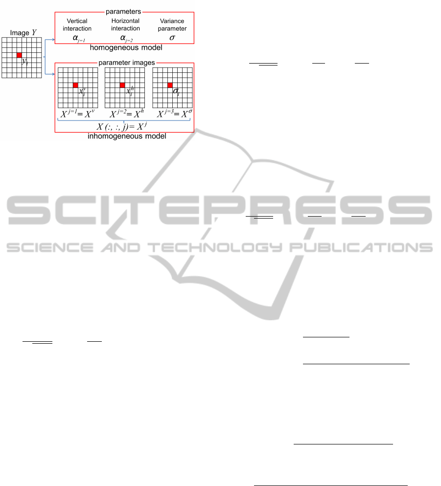
Figure 1: Parameters associated with the GMRF models.
neighborhood system is considered. Therefore three
types of model parameters are involved in character-
izing the model, namely, horizontal and vertical in-
teraction parameters and the variance parameter. In
the inhomogeneous model, for each type of parame-
ter, for example the vertical interaction parameter, the
parameter image is given by X
v
which represent the
vertical interaction parameter values x
v
i
at each pixel
i ∈ Ω of the spatial domain.
Once the parameters are defined and are assumed
to be known, then the likelihood of the texture image
Y can be written as,
p(Y |X ) =
∏
i
1
q
2πσ
2
i
exp



−
1
2σ
2
i
y
i
−
∑
j∈
˜
N
i
x
j
i
¯y
j
!
2



(3)
Here the formulation of the inhomogeneous model
involves many model parameters compared to spa-
tially constant model formulation. But the estimation
process can be easily parallelized using the coding
scheme (Petrou and Sevilla, 2006) for a much faster
estimation process.
The model parameter values on a parameter image
will be repetitive according to the pattern repetition.
Therefore the unique model parameter values on the
parameter image correspond to the parameter values
on one texel element. However, the size of the texel
is not clearly identifiable in many types of textures,
therefore we have considered a region of the texture,
Ω as above. Then the distribution of the repetitive
model parameters can be used to formulate the texture
features.
Next we look at the prior distribution of the model.
The prior model on parameters can also be defined
as a GMRF on the parameter space. Here we limit
our focus to smoothing priors. Alternately, any prior
knowledge available on the location dependence of
parameters could be associated to the prior model.
The prior model for interaction parameters can be
written as,
p(X
j
|γ) =
∏
i
1
p
2πγ
2
exp



−
1
2γ
2
x
j
i
−
1
|N
i
|
∑
r∈N
i
x
j
r
!
2



(4)
N
i
is the neighbors of site i on the parameter image
X
j
. |N
i
| is the number of neighbors. The above prior
model is defined for j = 1,...,R. i.e. for interaction
parameters. γ
2
is the hyper variance parameter of spa-
tially varying model parameters. It is considered that
the value of γ is same for any interaction parameter
X
j
for j = 1,...,R. The prior model for the variance
parameter is,
p(X
R+1
|δ) =
∏
i
1
√
2πδ
2
exp



−
1
2δ
2
σ
i
−
1
|N
i
|
∑
r∈N
i
σ
r
!
2



(5)
where δ is a constant and σ
i
is same as x
R+1
i
and
is used for better readability (figure 1).
2.3 Bayesian Formulation
The posterior density for the inhomogeneous texture
model can be written as follows.
p(X,γ,δ|Y) =
p(X,γ,δ,Y )
p(Y )
=
p(Y |X ,γ,δ)p(X|γ, δ)p(γ, δ)
p(Y )
We assume the conditional independence between
various variables to simplify the above expression, in-
cluding the independence between hyper parameters,
γ and δ. The posterior density can be then written as,
p(X, γ, δ|Y ) =
p(Y |X )p(X|γ, δ)p(γ)p(δ)
p(Y )
=
p(Y |X )
R
∏
j=1
p(X
j
|γ) p(X
R+1
|δ)p(γ)p(δ)
p(Y )
(6)
Since there is no prior knowledge about γ and δ
uniform distributions for p(γ) and p(δ) are assumed.
All the other densities are defined as in section 2.2.
It is important to mention about the local condi-
tional models of the joint models in (3), (4) and (5).
A local conditional model tells us about how a pixel
depends on its neighbors. Even though we use the
global models in MCMC estimation, when calculat-
ing acceptance probabilities, all the terms will cancel
out, except terms associated to the local models due
AnInhomogeneousBayesianTextureModelforSpatiallyVaryingParameterEstimation
141

to Markovian property given a symmetric proposal
distribution. The local conditional models of (3), (4)
and (5) intuitively become the expressions without the
product symbol. But in this study we use a slightly al-
tered local model for (3) as below.
p(y
i
|X
i
) =
m
∏
r
1
q
2πσ
2
i
exp



−
1
2σ
2
i
y
r
−
∑
j∈
˜
N
r
x
j
i
¯y
j
!
2



(7)
m represents the number of immediate neighbors
of site i, for example eight neighbors around i. This
expresses that probability of a pixel value not only
depends on its neighborhood but also on near by m
pixels and their neighbors. It is a localized version of
the likelihood of m samples. Therefore σ
2
i
represents
the variance considering m local samples which is a
localized variation at site i. Prior to using m local
samples their sample mean is set to zero.
2.4 MCMC estimation
Following (Aykroyd, 1998) we also use the
Metropolis-Hastings (MH) algorithm for parameter
estimation. Therefore finding normalizing constant
of posterior distribution in (6) is no longer needed.
Coding scheme (Petrou and Sevilla, 2006) is used
to estimate parameters in parallel on each X
j
, j =
1,...,R + 1. Each type of parameters including γ and
δ are sequentially estimated in turns. Approach to the
estimation of various groups of model parameters is
the same.
Let model parameters be represented by Θ where
Θ = {X,γ,δ}. Let the parameter being considered
be θ
i
. A proposed new value is selected from the
proposal distribution q(θ
0
i
|θ
i
). The set of parame-
ters containing the proposed value is given by Θ
0
=
{θ
1
,...,θ
i−1
,θ
0
i
,θ
i+1
,...,θ
|Ω|(R+1)+2
}. The proposed
value of parameter is accepted and then updated with
the acceptance probability,
min
(
1,
p(Θ
0
|Y )q(θ
0
i
|θ
i
)
p(Θ|Y )q(θ
i
|θ
0
i
)
)
(8)
Otherwise it is rejected and the previous value is
retained. Doubly exponential distribution centered on
the current value is used as the proposal distribution.
The scale parameter of proposal distribution is chosen
by trial and error technique. Since the proposal distri-
bution is symmetric the ratio q(θ
0
i
|θ
i
)/q(θ
i
|θ
0
i
) in (8)
is canceled out. The values of X
R+1
, γ and δ are cho-
sen to be positive all the time.
Many terms of the ratio in (8) will cancel out due
to Markovian property. This leads to vastly simplified
expressions. To avoid numerical overflow log value
of posterior ratio is used. The Markov chain is devel-
oped with the accepted samples chosen according to
the acceptance probability. The convergence of the
chain is monitored graphically. When the chain is
converged the average of samples laying outside the
burn-in period are used as the expected value of the
corresponding parameter.
Once the model parameters are estimated in this
way, their spatial distributions constructed by normal-
ized histograms can be used to formulate discrimina-
tive texture features.
3 RESULTS AND DISCUSSION
The Bayesian framework for the textures proposed
here can be used to extract spatially varying model
parameters and their spatial distributions can be used
as effective texture features for classification.
In this paper, the focus is limited to the first order
neighborhood system of GMRFs. Therefore three dif-
ferent types of model parameters, namely horizontal
interaction parameter, vertical interaction parameter
and variance parameter characterize the model.
Spatially varying model parameters are estimated
by sampling the proposed posterior probability distri-
bution in (6) and then taking the expected values of
the samples excluding the burn-in period. MH algo-
rithm is performed on each individual site to sample
and estimate the parameters at that location. The cod-
ing scheme (Petrou and Sevilla, 2006) is used to speed
up the process where instead of visiting each site in
the image sequentially, a batch of pixels belonging to
the same code is updated in parallel.
Each Markov chain is run for 2000 iterations. The
first 500 samples are considered as the burn-in period.
Rest of the samples are used to calculate the expected
value of the parameter.
The scale parameters of doubly exponential pro-
posal distributions are set by trial and error method
for each type of model parameters. For Markov chain
updates of interaction parameters, X
j
, j = 1,... , R the
scale parameter is 0.05 and for the variance parame-
ter X
R+1
it is 0.1. For super parameters γ and δ, 0.05
and 0.1 are used respectively. The number of local
samples for the likelihood model, m is restricted to
the five nearest samples in the proximity of consid-
ered site. This parameter setting is kept constant for
all the experiments unless stated otherwise.
In figure 2 examples of estimated parameter im-
ages (expected values) achieved using the inhomo-
geneous Bayesian framework are shown. Figure 2a
has two texture regions and corresponding horizon-
ICPRAM2014-InternationalConferenceonPatternRecognitionApplicationsandMethods
142

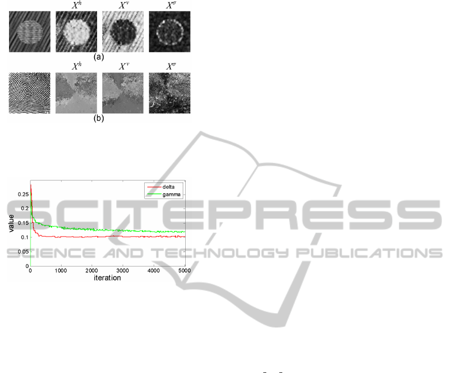
Figure 2: Parameter images obtained by inhomogeneous
Bayesian framework for parameter estimation. X
h
- hor-
izontal interaction parameter, X
v
- vertical interaction pa-
rameter, X
σ
- variance parameter
Figure 3: Markov Chains of δ and γ parameters for image
in figure 2a.
tal and vertical interaction parameter images illustrate
the spatially varying nature of the estimated model pa-
rameters. The variance parameter clearly indicates a
higher variance near the boundary between the two
texture regions. The pattern inside the circular region
in figure 2a has more noteworthy horizontal interac-
tions. The corresponding horizontal interaction pa-
rameter image has higher interaction parameter val-
ues in respective region. Also the pattern outside the
circular region has a directional pattern closer to the
vertical axis. Hence the corresponding vertical inter-
action parameter has higher interaction values outside
the circular region.
Figure 2b shows a partial finger print. The spa-
tially varying parameters are not made rotational or
scale invariant here. Therefore the corresponding spa-
tially varying parameters capture the directional dif-
ferences in the patterns of the finger print. In general,
by looking at figure 2 it can be concluded that spa-
tially varying model parameters carry more informa-
tion about the texture.
The Markov chains of super parameters γ and δ of
figure 2a are shown in figure 3. These chains graph-
ically indicate the convergence roughly after 200 it-
erations. Therefore the burn-in period and number of
iterations mentioned earlier are suitable values.
The local distributions of these spatially varying
parameters can be used to discriminate texture re-
gions. An evaluation of spatial distributions of spa-
tially varying parameters is illustrated in figure 4.
Four textures are used and their corresponding spa-
tially varying parameter images are obtained and con-
verted into normalized histograms with 50 bins. The
parameter image values are modified to lie between
the range 0 to 255 before constructing the histograms.
This normalization is done for illustration purposes
only. The intensity histograms of the four textures are
given in figure 4c.
According to figure 4c it can be seen that discrim-
ination power of the intensity histogram is quite low
for these four textures. But the histograms of param-
eter images represent substantial differences in there
distributions. The interaction parameter histograms in
figure 4d and e show a negative correlation between
the distributions for a texture. Here we have only
two interaction parameters in the model. Therefore,
when the horizontal interaction is dominant, vertical
interaction of the respective texture is much insignifi-
cant. However, these distributions of spatially varying
model parameters can be used as a discriminative tex-
ture feature in texture analysis.
3.1 General Texture Classification
We perform texture classification using two datasets
namely BRODATZ, a random subset of Brodatz
dataset (Valkealahti and Oja, 1998) comprising 32
Brodatz textures (Brodatz, 1996) and OUTEX, the full
OUTEX TC 00001 dataset having 24 OUTEX tex-
tures (Ojala et al., 2002). Each dataset has 20 samples
per class. Prior to feature extraction all the images
are pre-processed using histogram equalization. Next,
parameter estimation is carried out and the distribu-
tions of spatially varying parameters are constructed
by normalized histograms.
The classification experiments are performed us-
ing equal sizes of training and test datasets randomly
partitioned to have equal class proportions. The ex-
periment is repeated 100 times with different train-
ing and test sets. Accuracies reported here are the
mean accuracy of 100 iterations and its standard devi-
ation. Classification is performed using nearest neigh-
bor classifier with absolute difference distance metric.
The accuracies are given in table 1. The pro-
posed inhomogeneous model based feature extrac-
tion is referred to as IBMF which stands for ‘Inho-
mogeneous Bayesian Model based Features’. The
feature extraction based on homogeneous Bayesian
model is labeled as HBMF which stands for ‘homo-
geneous Bayesian Model based Features’. Four other
methods have been used for performance compari-
AnInhomogeneousBayesianTextureModelforSpatiallyVaryingParameterEstimation
143

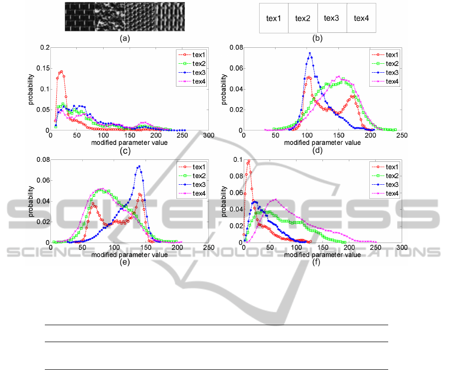
Figure 4: Histogram comparison. (a) image comprising four textures, (b) texture labels, and (c) intensity histograms. His-
tograms of spatially varying parameter images (d) histograms of X
h
(e) histograms of X
v
(f) histograms of σ of each texture.
Table 1: Accuracy comparison with other methods. First order neighborhood system is used. bins = 50 is used for IBMF and
PL methods.
dataset IBMF HBMF PL TGMRF LBP
BRODATZ 88.2 ±1.54 37.9 ±2.19 81.0 ±1.13 40.7 ±2.02 89.7 ±1.90
OUTEX 87.0 ±1.69 31.7 ±2.19 83.1 ±1.99 40.7 ±2.59 79.5 ±2.10
son. The method PL is based on the spatially varying
model parameters estimated using small model esti-
mation which uses LSE (Dharmagunawardhana et al.,
2012). TGMRF is the traditional GMRF feature ex-
traction method (Manjunath and Chellappa, 1991).
The method LBP is based on rotational invariant uni-
form local binary patterns (Ojala et al., 2002) and
are implemented using (Heikkila and Ahonen, 2012).
Only the LBP histograms from (P=8,R=1) are used to
get roughly similar neighborhood representations as
the GMRF setting where the first order neighborhood
system is used.
It is clearly observed that the texture features
based on spatially varying parameters significantly
perform better than spatially constant parameters (ta-
ble 1). Comparative studies by other authors have also
reported the reduced discriminative ability of the spa-
tially constant MRF features (Ojala et al., 2001; Had-
jidemetriou et al., 2003). Note that we have only used
first-order GMRFs here. By increasing the neighbor-
hood size accuracies can be further improved.
Furthermore, it is observed that the IBMF has bet-
ter accuracy compared to PL method based on LSE
(table 1). A comparison between accuracies obtained
in 100 iterations from LBP and PL methods with
IBMF are shown in figure 6. The IBMF features per-
form better in most of the trials except for the BRO-
DATZ dataset with LBP method (figure 6a). Here, the
results are comparable with LBP method. However, in
certain applications, for example medical image pro-
cessing, when prior knowledge about pathology local-
ization is available or smoothing priors for noise re-
duction is reasonably important, IBMF can make use
of these additional information about the problem in
hand through prior distribution unlike with LBP.
In the present study, we have employed the local
smoothing priors for IBMF method. Therefore by us-
ing appropriate prior information, IBMF features can
perform better than the simple least square estimation
based PL features.
ICPRAM2014-InternationalConferenceonPatternRecognitionApplicationsandMethods
144

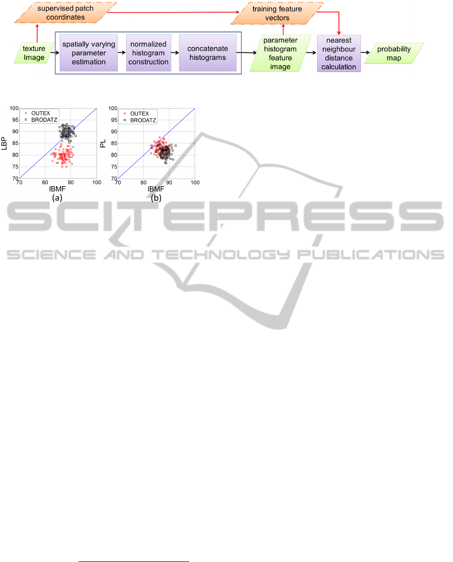
Figure 5: Supervised texture segmentation method.
Figure 6: Comparison between accuracies obtained from
IBMF with LBP and PL in 100 trials. (a) IBMF with LBP
(b) IBMF with PL.
3.2 Texture Segmentation
We perform supervised texture segmentation using
IBMF features on gray scale natural images from
Berkeley dataset (Martin et al., 2001) and Alpert
dataset (Alpert et al., 2007). After extracting spatially
varying parameters of the image, a sliding window of
size b = 21pxls is used to construct the local param-
eter histograms at each pixel. The process is super-
vised in the sense that a supervised patch of interested
texture, extracted from the input image itself, is fed
into the system to calculate training data. The method
is illustrated in figure 5.
First the coordinates of the supervised patch area,
entered by the user, are stored and then the feature
extraction for the texture image is conducted as previ-
ously discussed. Once the features are extracted for
all pixels, the stored coordinates are used to select
the training feature vectors from the feature image.
Next, L1 norm distance between each feature vec-
tor to the nearest training feature vector is calculated.
These distance measures are converted into probabil-
ity values according to the following equation. Let
supervised patch area containing texture of interest be
Ω
t
⊆ Ω.
p
i
(ω/h
k
,k ∈Ω
t
) =
exp{−D
min
(h
i
,h
k
)
2
}
max
i∈Ω
(exp{−D
min
(h
i
,h
k
)
2
})
(9)
where local parameter histogram feature vector at
a pixel i is denoted by h
i
and D
min
is the L1 norm
distance of a feature vector to its nearest training fea-
ture vector. p
i
(ω/h
k
,k ∈ Ω
t
) gives the probability of
a pixel at location i belonging to the texture of inter-
est, ω. The probability map calculated in this man-
ner is shown in figure 7. The probability map is then
thresholded using a suitable threshold value to ac-
quire the texture of interest (figure 7). These results
are achieved using the first order neighborhood sys-
tem (horizontal and vertical interaction parameters)
for IBMF formulation. If higher order neighborhood
systems are used, the results can be further improved.
However, here we mainly focus on introducing the
theory of IBMF and limit our interest to the first order
neighborhood system.
The region boundaries obtained by thresholding
the probability map gives a satisfactory texture seg-
mentation (figure 7). Segmentation process can be
further improved using other suitable advanced seg-
mentation methods such as clustering techniques or
active contours (Mahmoodi and Gunn, 2011).
4 CONCLUSIONS
We have proposed a novel GMRF based Bayesian tex-
ture model characterized by spatially varying model
parameters for texture feature extraction. The hier-
archical Bayesian formulation of the posterior model
and the parameter estimation process are compre-
hensively explained. The distributions of estimated
model parameters are used as an effective texture fea-
ture in texture classification and segmentation. The
results reveal that the proposed method outperform
the texture features based on spatially constant model
parameters of GMRF and LSE based spatially varying
parameters. It can be further concluded that in statis-
tical model based texture feature extraction, spatially
varying parameters are more suitable, capturing both
spatial pixel dependencies and structural properties of
the texture. The Bayesian formulation enables inte-
gration of prior knowledge to the spatially varying pa-
rameter estimation process and further improves the
features based on them. Furthermore we have per-
formed successful supervised texture segmentation on
natural images to segment the areas of a given tex-
ture of interest, using probability maps and the simple
thresholding technique.
AnInhomogeneousBayesianTextureModelforSpatiallyVaryingParameterEstimation
145

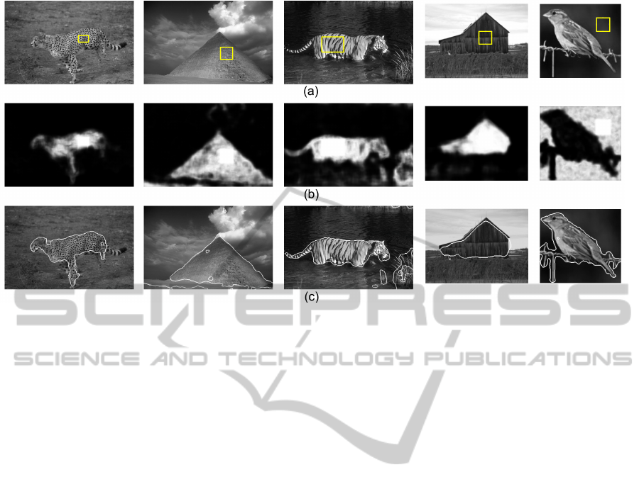
Figure 7: Supervised texture segmentation results. (a) original images with the supervised patch selected by the user. (b)
probability maps. (c) boundaries obtained by thresholding the probability map. Note: first order neighborhood system is used
for IBMF.
REFERENCES
Alpert, S., Galun, M., Basri, R., and Brandt, A. (2007). Im-
age segmentation by probabilistic bottom-up aggrega-
tion and cue integration. In Proc. of the IEEE Conf.
Computer Vision and Pattern Recognition.
Aykroyd, R. (1998). Bayesian estimation for homogeneous
and inhomogeneous gaussian random fields. IEEE
Trans. on pattern analysis and machine intelligence,
20:533–539.
Brodatz, P. (1996). Textures: A Photographic Album for
Artists and Designers. New York: Dover.
Chellappa, R. and Chatterjee, S. (1985). Classification of
textures using Gaussian Markov random fields. IEEE
Trans. on Acoustics Speech and Signal Processing,
33(4):959–963.
Dharmagunawardhana, C., Mahmoodi, S., Bennett, M., and
Mahesan, N. (2012). Unsupervised texture segmen-
tation using active contours and local distributions
of Gaussian Markov random field parameters. In
Proc. British Machine Vision Conference, pages 88.1–
88.11.
Hadjidemetriou, E., Grossberg, M. D., and Nayar, S. K.
(2003). Multiresolution histograms and their use for
texture classification. In Int’l Workshop on Texture
Analysis and Synthesis, Nice, France.
Heikkila, M. and Ahonen, T. (2012). Uni-
form Local Binary Patterns: Matlab code.
http://www.cse.oulu.fi/CMV/Downloads/LBPMatlab.
Li, S. Z. (2009). Markov Random Field Modeling in Im-
age Analysis. Springer-Verlag London Ltd, 3rd edn
edition.
Mahmoodi, S. and Gunn, S. (2011). Snake based unsuper-
vised texture segmentation using Gaussian Markov
random field models. In Proc. 18th IEEE Int’l Conf.
Image Processing, pages 1–4.
Manjunath, B. S. and Chellappa, R. (1991). Unsuper-
vised texture segmentation using Markov random
field models. IEEE Trans. on pattern analysis and
machine intelligence, 13(5):478–482.
Martin, D., Fowlkes, Tal, D., and Malik, J. (2001). A
database of human segmented natural images and its
application to evaluating segmentation algorithms and
measuring ecological statistics. In Proc. 8th Int’l
Conf. Computer Vision, pages 416–423.
Ojala, T., Pietikainen, M., and Maenpaa, T. (2002). Mul-
tiresolution gray-scale and rotation invariant texture
classification with local binary patterns. IEEE Trans.
on pattern analysis and machine intelligence, 24:971–
987.
Ojala, T., Valkealahti, K., Oja, E., and Pietik
¨
ainen, M.
(2001). Texture discrimination with multidimensional
distributions of signed gray-level differences. Pattern
Recognition, 34:727–739.
Petrou, M. and Sevilla, P. G. (2006). Image Processing,
Dealing with Texture. John Wiley & Sons Ltd.
Valkealahti, K. and Oja, E. (1998). Reduced multidimen-
sional co-occurrence histograms in texture classifica-
tion. IEEE Trans. on Pattern Analysis and Machine
Intelligence, 20:90–94.
Zhao, Y., Zhang, L., Li, P., and Huang, B. (2007). Classi-
fication of high spatial resolution imagery using im-
proved Gaussian Markov random-field-based texture
features. IEEE Trans. on Geoscience and Remote
Sensing, 45(5):1458–1468.
ICPRAM2014-InternationalConferenceonPatternRecognitionApplicationsandMethods
146