
An Efficient Solution to 3D Reconstruction from Two Uncalibrated
Views under SV Constraint
Shuyang Dou
1
, Hiroshi Nagahashi
2
and Xiaolin Zhang
3
1
Department of Information Processing, Tokyo Institute of Technology,
4259 Nagatsuta-cho, Midori-ku, Yokohama, Kanagawa 226-8503, Japan
2
Imaging Science and Engineering Laboratory, Tokyo Institute of Technology,
4259 Nagatsuta-cho, Midori-ku, Yokohama, Kanagawa 226-8503, Japan
3
Precision and Intelligence Laboratory, Tokyo Institute of Technology,
4259 Nagatsuta-cho, Midori-ku, Yokohama, Kanagawa 226-8503, Japan
Keywords: 3D Reconstruction, Uncalibrated Views, Focal Length Estimation, Standard Vergence.
Abstract: In this paper, an efficient solution is proposed to the problem of 3D reconstruction from two uncalibrated
views under Standard Vergence (SV) constraint. This solution consists of three core steps: firstly, set up the
camera configuration according to SV constraint; secondly, estimate camera's focal length and relative pose
between two views; lastly, reconstruct the scene optimally by minimizing reprojection error. By analysing
the degenerated camera motion under SV constraint, a novel method for efficiently estimating camera's
focal length and relative pose is proposed. Both synthetic and real data experiments showed that this new
method could provide close estimation, which resulted in fast convergence in the most time-consuming step
of final optimization. The main contribution of this paper is that it is the first time to introduce SV constraint
into 3D reconstruction problem, and an efficient solution which utilizes this constraint is proposed.
1 INTRODUCTION
Reconstructing the three dimensional (3D) model of
scene has been a big challenge for many years in
Computer Vision. A lot of methods for this problem
were proposed. For example, Goesele et al. (2006)
presented a robust multi-view stereo algorithm.
Alexiadis et al. (2013) provided a real-time solution
by using a multiple-Kinect capturing system.
Besides, reconstruction from two uncalibrated views
is an attracting approach. The reason for this is that
only two views are used, neither prior camera
calibration nor any knowledge about the scene is
necessary. Thus, it is very cheap and easy to
implement this method with just a camera.
In such an approach, camera needs to be
automatically calibrated. This problem can be
simplified to focal length estimation when semi-
calibrated camera is used. This is a reasonable
assumption for modern cameras. Many approaches
of focal length estimation have been proposed
during past years. Hartley (1992, in Kanatani et al.,
2006) provided a solution by using the singular
value decomposition (SVD) technique. Then, Pan et
al. (1995a, b, in Kanatani et al., 2006) proposed a
new method by solving cubic equations. After that,
Bougnoux (1998, in Kanatani et al., 2006) provided
a closed form to estimate the focal length. Recently,
Pernek and Hajder (2013) presented a novel solution
by transforming this problem into the generalized
eigenvalue problem introduced in Kukelova et al.
(2008, in Pernek and Hajder, 2013). Besides,
Stewenius et al. (2005) and Hartley and Li (2012)
also proposed minimal approaches. Many methods
will degenerate in fixed configuration, in which two
optical axes intersect with each other. In order to
deal with this difficulty, Brooks et al. (1998) and
Kanatani and Matsunaga (2000) provided different
solutions. However, these methods usually could
only provide results with more deviations than
traditional camera calibration methods, like the
popular method proposed by Zhang (2000). As a
result, reconstruction using these methods often
converges slowly and lacks for accuracy.
In this paper, an efficient solution for 3D
reconstruction from two uncalibrated views is
presented by introducing an additional constraint on
camera motion, called Standard Vergence (SV)
664
Dou S., Nagahashi H. and Zhang X..
An Efficient Solution to 3D Reconstruction from Two Uncalibrated Views under SV Constraint.
DOI: 10.5220/0004748006640671
In Proceedings of the 9th International Conference on Computer Vision Theory and Applications (VISAPP-2014), pages 664-671
ISBN: 978-989-758-009-3
Copyright
c
2014 SCITEPRESS (Science and Technology Publications, Lda.)

constraint. Under this constraint, the camera motion
degenerates to a special planar case. Based on
analyzing the geometric meaning of SV constraint, a
new method is proposed for estimating camera's
focal length and relative pose. Both synthetic and
real data experimental results showed that this new
method could provide very close estimations, and by
using these initial values, a fast and accurate
reconstruction solution could be achieved.
The following sections are organized like this:
section 2 introduces fundamentals of SV constraint,
section 3 explains the three core steps of our
solution, section 4 shows the details of both
synthetic and real data experiments, section 5
concludes the paper.
2 STANDARD VERGENCE
FUNDAMENTALS
In order to explain the SV constraint more
intuitively, a few useful terms will be described. Fig.
1 shows a fixed camera configuration. For each
camera coordinate system, there are a vertical axis
( and ′ for camera and ′
respectively) and a horizontal plane (
and ′′ for and ′ respectively). Two
optical axes, and ′, intersect at
point , called the optical intersection. The angle
made by two optical axes is called the convergence
angle. Furthermore, if the two distances from the
optical intersection to each camera centre are same,
then this case is called an isosceles triangle
configuration.
Figure 1: Fixed configuration.
SV constraint consists of two conditions: the first
one is called horizontal condition, both of the two
cameras share the same horizontal plane, which
implies that there is no horizontal distortion between
two views; the second one is called intersection
condition, the two optical axes intersect with each
other, which is fair to say that it must be a fixed
configuration. By using Fig. 1, the horizontal
condition is equivalent to say that and
′′ must be the same plane, on the other
hand, the intersection condition states that
and ′ must intersect at some point .
From these two conditions, the geometric
meaning of SV constraint can be easily revealed as:
the camera can only be moved and rotated on its
horizontal plane. In this case, the camera motion
degenerates to a special planar motion called SV
motion.
SV motion was first proposed by Zhen et al.
(2010). It originally comes from analysing the
motion between two eyes of human beings. Each eye
can be seen as a camera, thus, two eyes constitute a
binocular system. It is easy to verify that the motion
between two eyes obeys the intersection condition,
because they are always focused on the target.
Furthermore, the horizontal condition is also
satisfied. If horizontal distortion exists between the
two images captured by two eyes, the brain will be
confused and unpleasant feeling will be felt.
Though SV motion is very familiar to us human
beings, it is rarely used in 3D reconstruction
problem. On the contrary, arbitrary or parallel
binocular systems are currently much more widely
used. This paper, for the first time, introduces SV
constraint into 3D reconstruction problem. Because
of the special degenerated form of camera motion
under SV constraint, the problem becomes much
simpler than general cases. Our new method for
estimating camera’s focal length and relative pose
directly comes from this important observation.
Figure 2: Different types of camera configuration.
Table 1: Applicable ranges for different focal length
estimation methods.
Method Applicable range
General method, like
(Bougnoux, 1998)
General configuration
except fixed configuration
Degenerated method, like
(Kanatani and Matsunaga,
2000)
Fixed configuration except
isosceles triangle
configuration
New method proposed in
this paper
SV motion
AnEfficientSolutionto3DReconstructionfromTwoUncalibratedViewsunderSVConstraint
665
Many focal length estimation approaches, like
(Bougnoux, 1998), will degenerate in fixed
configuration, so they are not applicable to SV
motion. Kanatani's method (Kanatani and
Matsunaga, 2000) can handle the fixed configuration
well. However, their method will degenerate in
isosceles triangle case, which is a special case of SV
motion. A new method is proposed in this paper
which can handle all cases of SV motion. The
applicable ranges for these methods are compared in
Fig. 2 and Table 1.
3 PROPOSED SOLUTION
Three reasonable assumptions are necessary for the
proposed solution: firstly, both of the two cameras
are semi-calibrated, this is equivalent to say that
except the focal length all the other intrinsic camera
parameters are already known, this assumption is
appropriate for modern cameras; secondly, the two
cameras have similar or same focal length, which
can be easily satisfied by moving one camera to
different viewpoints without changing the zoom and
focus values, or using a binocular system with two
cameras of same series and synchronizing their
zoom and focus values; lastly, the camera motion
between two views must obey SV constraint.
According to the geometric meaning of SV, the
camera configuration is easily set up to satisfy SV
constraint like this: install the camera on a tripod and
adjust it to be horizontal, then find a horizontal
ground plane and place the equipment on it. The
motion, which is composed by translating and
rotating this equipment freely on the ground without
changing the tripod's height, as well as camera's
zoom and focus value, is SV motion. Thus, with a
camera, a tripod and a horizontal ground plane, SV
motion can be easily achieved manually.
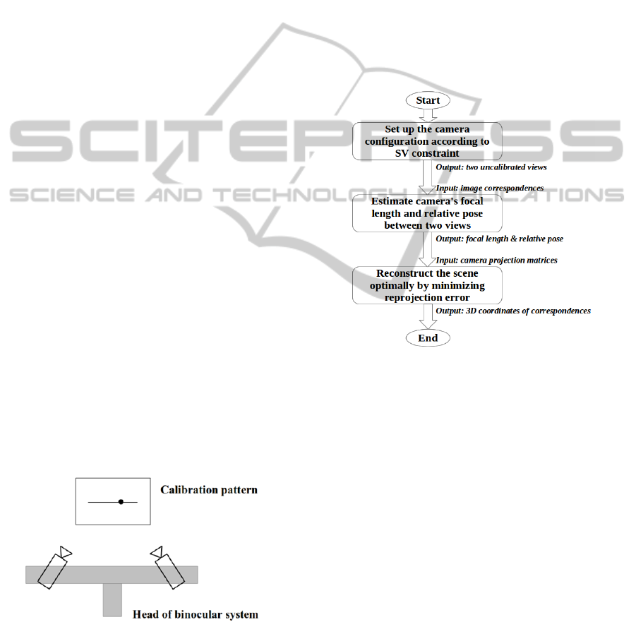
Figure 3: Calibration of binocular system.
For the case of using a binocular system, SV
motion can be achieved by calibrating the position
of each camera. In Fig. 3, a simple calibration
pattern of a line and an arbitrary marked point on it
is used. Each camera is adjusted accordingly so that
the projection of the marked point is located at the
image centre, and the projection of the line is
parallel to the image’s horizontal axis. Finally, the
camera motion becomes a SV motion. Note that,
after this calibration step, each camera can only be
rotated about its vertical axis. However, the head of
the binocular system can be freely moved.
It is more challenging to satisfy SV constraint for
a fully active binocular system, in which each
camera can be moved freely. The basic idea is
analysing and eliminating the horizontal distortion
between two views. However, no details about such
algorithm will be discussed in this paper.
Figure 4: Flow chart of proposed solution.
The flow chart of proposed solution is showed in
Fig. 4. It consists of three core steps: firstly, set up
the camera configuration according to SV constraint,
the method described previously is implemented in
this step; secondly, estimate camera's focal length
and relative pose between two views, this is done by
using a new method which will be explained in
detail later; lastly, reconstruct the scene optimally by
minimizing reprojection error, this step can be
sequentially divided into two stages: at first, a quick
linear reconstruction is given by using the
triangulation method; then, the reconstruction is
refined by a non-linear optimization step using
sparse Levenberg-Marquardt (LM) method (Hartley
and Zisserman, 2004: 602). There are other works,
like matching correspondences between the first and
second step, need to be done in this solution.
However, no discussion on these will be developed
here because they are not focus points of this paper.
The new method for estimating camera’s focal
VISAPP2014-InternationalConferenceonComputerVisionTheoryandApplications
666

length and relative pose used in step 2 is directly
deduced by utilizing the degenerated form of camera
motion. Usually, a 33 orthogonal matrix and a
3-element vector are used to parameterize the
camera's relative pose. In SV motion, camera only
rotates about its vertical axis, so only one parameter,
the convergence angle, is sufficient to describe the
rotation. Thus, the degree of freedom (DOF) of is
reduced from 3 to 1. Meanwhile, the translation only
happens on camera's horizontal plane, so the
translation element of along the vertical optical
axis is zero. Thus, vector has DOF of 2. As a
result, under SV motion, matrix and vector will
degenerate to the following forms:
0
0
1
0
0
(1)
0
(2)
where represents the convergence angle.
The essential matrix will have a special
degenerated form as shown in eq. (3) by substituting
eq. (1) and (2) into its decomposition form.
Now, by using eq. (3), the relationship between
the fundamental and essential matrices provided by
Hartley and Zisserman (2004: 257) can be developed
as eq. (4), where and ′ are camera calibration
matrices, with same unknown focal length value
and known principle point located at
,
,
,
respectively.
0
0
0
0
0
0
0
1
0
0
0
0
0
0
0
0
0
0
0
0
(3)
The fundamental matrix can be directly
estimated from correspondences. Thus, from eq. (3)
and (4), it is easy to deduce eq. (5) to (9), which give
a solution to , and .
(5)
1
(6)
(7)
(8)
(9)
From eq. (7) to (9), it is easy to see that this
method will degenerate only when is zero. In this
case, two optical axes will be parallel to each other.
This is an obvious violation of the intersection
condition of SV constraint. So, under SV constraint,
this method can always give a solution. However,
due to image noises, mismatching of
correspondences or other reasons, may be
greater than 1, and consequently will take
imaginary value, in which case this method will fail.
Thus, it can be concluded that this method is
applicable to any SV motion, though sometimes
imaginary result might be given due to noises or
other reasons.
4 EXPERIMENTS
4.1 Comparison Experiment
The goal for this experiment is to compare the
efficiency of our new method with Kanatani's
method (Kanatani and Matsunaga, 2000) on task of
focal length estimation. The source code of their
method is provided by Yamada et al. (2009). Totally
211 3D points from a part of a sphere surface,
generated by ParaView (Kitware Inc. et al., 2013),
are projected to each image plane (Fig. 5). The
position and orientation of each camera are adjusted
by two parameters as shown in Fig. 6: the
convergence angle and the distance ratio . It is
easy to verify that each pair of and can
uniquely define a triangle ∆′up to scale. Thus,
any SV motion can be achieved by setting proper
values for and .
′
1
0
0
1
0
0
0
0
0
0
0
1
0
0
0
1
0
0
0
(4)
AnEfficientSolutionto3DReconstructionfromTwoUncalibratedViewsunderSVConstraint
667
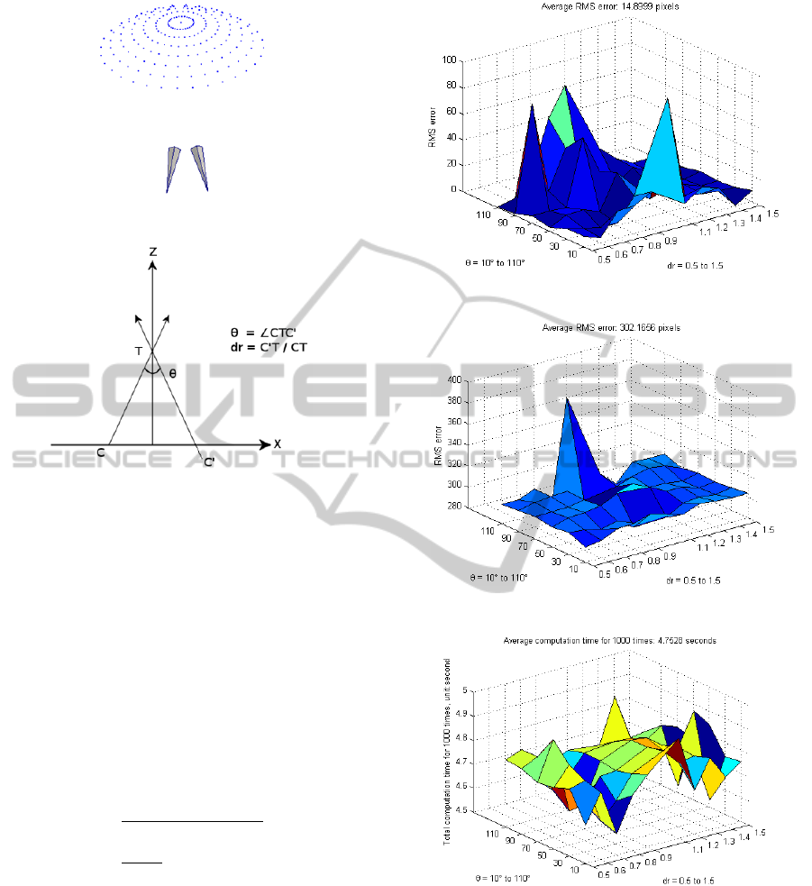
Figure 5: 3D points and cameras.
Figure 6: Camera configuration parameters.
In this experiment, the convergence angle was
chose from 10° to 100° with step of 20°. The
distance ratio was chose from 0.5 to 1.5 with step
of 0.1. The value 1.0 was skipped, because this is an
isosceles configuration, in which case Kanatani's
method (Kanatani and Matsunaga, 2000) will
degenerate.
The true focal length was
̅
1000 pixels for
both cameras. A Gaussian noise with standard
derivation 0.5 pixels was added to each image.
Each configuration was tested 1000 times. The Root
Mean Squares (RMS) error, which is defined as eq.
(10), and computation time for each method is given
in Fig. 7 to 10.
1
1000
(10)
The average RMS error for our method was about
14.8999 pixels, while 302.1656 pixels for Kanatani's
method (Kanatani and Matsunaga, 2000). The
reason for this is that only the intersection condition
is used in their method, while the horizontal
condition is also considered in our method. In other
words, our method is only valid for SV motion, a
much more specified applicable range than their
method. It is common that a solution to a highly
specified problem gain more accuracy than a
solution to a more general problem.
Figure 7: RMS error of our method.
Figure 8: RMS error of Kanatani's method.
Figure 9: Computation time of our method.
The average computation time for 1000 times
was 4.7528 seconds and 75.1425 seconds for our
method and Kanatani's method (Kanatani and
Matsunaga, 2000) respectively. The reason for
significant shortening of computation time is simple:
it only takes a few elementary calculations in our
method, while polynomial calculations are necessary
in their method.
In a conclusion, this experiment showed that
VISAPP2014-InternationalConferenceonComputerVisionTheoryandApplications
668
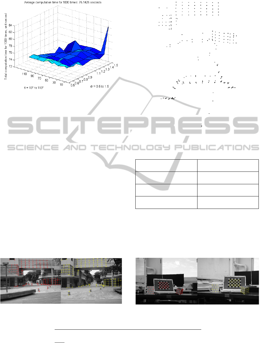
Figure 10: Computation time of Kanatani's method.
under SV constraint, our method is much more
efficient than Kanatani's method (Kanatani and
Matsunaga, 2000) for the task of focal length
estimation.
4.2 Real Scene Images Experiment
In this experiment, the efficiency of the proposed
solution for 3D reconstruction was test by using both
outdoor and indoor scene images. The camera
configuration method described in section 3 was
implemented. Totally 124 and 75 image
correspondences, for outdoor and indoor scenes
respectively, were selected manually, which were
considered to represent the geometric shape of the
scene well. Then, the 3D coordinate for each
coordinate was reconstructed by using the proposed
solution. Accuracy is represented by the RMS
reprojection error, which is defined as eq. (11),
where
,
and
,
are reprojected image
points,
,
and ′
,′
are manually selected
image points.
Figure 11: Manually selected correspondences (outdoor).
Figure 12: Two views of 3D points (outdoor).
Table 2: Optimization results (outdoor): reprojection error
and focal length estimation, units for all values are pixel.
RMS reprojection error
1st loop: 7.1573
2nd loop: 0.5174
Initial focal length
estimation
,
(1322.6, 1322.6)
Optimal focal length of
1st camera
(1322.5, 1322.8)
Optimal focal length of
2nd camera
(1180.9, 1319.3)
From Fig. 11 and 12, it can be easily confirmed
that the reconstructed shape of the building is
consistent to its real geometric shape. In Fig. 14, the
reconstructed two orthogonal faces of the magic
cube, and the curved surface of the cup represent
the shape of the objects well.
Figure 13: Manually selected correspondences (indoor).
1
248
′
′
′
′
(11)
AnEfficientSolutionto3DReconstructionfromTwoUncalibratedViewsunderSVConstraint
669

Figure 14: Two views of 3D points (indoor).
Table 3: Optimization results (indoor): reprojection error
and focal length estimation, units for all values are pixel.
RMS reprojection error
1st loop: 59.5622
2nd loop: 1.4326
3rd loop: 0.5576
Initial focal length
estimation
,
(3613.5, 3613.5)
Optimal focal length of
1st camera
(3620.6, 3652.6)
Optimal focal length of
2nd camera
(3646.6, 3410.2)
From the data showed in Table 2 and 3, it can be
known that the final reconstruction result is
reasonably high accurate, whose RMS reprojection
error is about 0.5 pixels. Meanwhile, the non-linear
optimization step converged very fast, which only
used 2 and 3 iterations for outdoor and indoor scenes
respectively. One of the reasons for this fast
convergence is highly accurate initial estimation for
focal length provided by our method.
For conclusion, both for outdoor and for indoor
environments, the new method can provide a close
estimation of focal length, which can dramatically
facilitate the most time-consuming optimization step
of 3D reconstruction.
5 CONCLUSIONS
In this paper, a special planar camera motion, called
SV motion, is introduced to the problem of 3D
reconstruction from two uncalibrated views. An
efficient solution to this problem is proposed. This
solution uses a new method for estimating camera’s
focal length and relative pose. Both synthetic and
real data tests showed that this method could provide
close initial values. As a result, the non-linear
optimization, which is the most time-consuming step
of 3D reconstruction, could converge very fast. In a
conclusion, an efficient solution is achieved to the
problem of 3D reconstruction from two uncalibrated
views under Standard Vergence (SV) constraint.
The main contribution of this paper is that it is
the first time to introduce SV constraint into 3D
reconstruction problem, and an efficient solution
which utilizes this constraint is proposed.
REFERENCES
Alexiadis, D. S., Zarpalas, D. and Daras, P. (2013) Real-
time, full 3-D reconstruction of moving foreground
objects from multiple consumer depth cameras. IEEE
Trans. Multimedia. 15(2):339-358.
Bougnoux, S. (1998) From projective to Euclidean space
under any practical situation, a criticism of self-
calibration. In: Proc. 6th Int. Conf. Comput. Vision,
Bombay, India, 790-796.
Brooks, M. J., de Agaptio, L., Huynh, D. Q. and Baumela,
L. (1998) Towards robust metric reconstruction via a
dynamic uncalibrated stereo head. Image Vision
Comput. 16(14):989-1002.
Goesele, M., Curless, B. and Seitz, S. M. (2006) Multi-
view stereo revisited. In: Proc. 2006 IEEE Comput.
Society Conf. Comput. Vision Pattern Recog. New
York, NY, USA. 2:2403-2409.
Hartley, R. I. (1992) Estimation of relative camera
positions for uncalibrated cameras. In: Proc. 2nd Euro.
Conf. Comput. Vision, Santa Margherita Ligure, Italy,
579-587.
Hartley, R. and Zisserman, A. (2004) Multiple view
geometry in computer vision. 2nd ed. Cambridge:
Cambridge University Press.
Hartley, R. and Li H. (2012) An efficient hidden variable
approach to minimal-cal camera motion estimation.
IEEE Trans. Pattern Anal. Mach. Intell. 34(12):2303-
2314.
Kanatani, K. and Matsunaga, C. (2000) Closed-form
expression for focal lengths from the fundamental
matrix. In: Proc. 4th Asian Conf. Comput. Vision,
Taipei, Taiwan, 1:128-133.
Kanatani, K., Nakatsuji, A. and Sugaya, Y. (2006)
Stabilizing the focal length computation for 3-D
reconstruction from two uncalibrated views. Int. J.
Comput. Vision. 66(2):109-122.
Kitware Inc., Sandia National Laboratories and
Computational Simulation Software, LLC. (2013)
ParaView (Version 4.0.1) [Computer program].
Available from http://www.paraview.org [Accessed 22
Jul. 2013].
Kukelova, Z., Bujnak, M. and Pajdla, T. (2008)
Polynomial eigenvalue solutions to the 5-pt and 6-pt
VISAPP2014-InternationalConferenceonComputerVisionTheoryandApplications
670

relative pose problems. In: Proc. British Machine
Vision Conf. Leeds, UK, 565-574.
Pan, H.-P., Brooks, M. J. and Newsam, G. N. (1995a)
Image resituation: initial theory. In: Proc. SPIE:
Videometrics IV, Philadelphia, PA, USA, 2598:162-
173.
Pan, H.-P., Huynh, D. Q. and Hamlyn, G. K. (1995b)
Two-image resituation: practical algorithm. In: Proc.
SPIE: Videometrics IV, Philadelphia, PA, USA,
2598:174-190.
Pernek, A. and Hajder, L. (2013) Automatic focal length
estimation as an eigenvalue problem. Pattern Recogn.
Lett. 24(9):1108-1117.
Stewenius, H., Nister, D., Kahl, F. and Schaffalitzky, F.
(2005) A minimal solution for relative pose with
unknown focal length. In: Proc. 2005 IEEE Comput.
Society Conf. Comput. Vision Pattern Recog. San
Diego, CA, USA, 2:789-794.
Yamada, K., Kanazawa, Y., Kanatani, K. and Sugaya, Y.
(2009) 3DRec-MATLAB [Computer Program].
Available from:
http://www.img.cs.tut.ac.jp/programs/index.html
[Accessed 22 Jul. 2013].
Zhang, Z. (2000) A flexible new technique for camera
calibration. IEEE Trans. Pattern Anal. Mach. Intell.
22(11):1330-1334.
Zhen, Z., Miao, Y., Sato, M. and Zhang, X. (2010)
Automatic 3D photographing device, In: Proc.
ASIAGRAPH, Tokyo, Japan, 4(1):235-237.
AnEfficientSolutionto3DReconstructionfromTwoUncalibratedViewsunderSVConstraint
671
