Effortless Scanning of 3D Object Models by Boundary Aligning and

Stitching

Susana Brand˜ao

1,2

, Jo˜ao P. Costeira

and Manuela Veloso

Instituto Superior T´ecnico, Universidade de Lisboa, Av Rovisco Pais, Lisboa, Portugal

Electrical and Computer Engineering Department, Carnegie Mellon University, Pittsburgh, U.S.A.

Computer Science Department, Carnegie Mellon University, Pittsburgh, U.S.A.

Keywords:

3D Object Modeling.

Abstract:

We contribute a novel algorithm for the digitation of complete 3D object models that requires little preparation

effort from the user. Notably, the presented algorithm, Joint Alignment and Stitching of Non-Overlapping

Meshes (JASNOM), completes 3D object models by aligning and stitching two 3D meshes by the boundaries

and does not require any previous registration between them. JASNOM only requirement is the lack of overlap

between meshes, which is simple to achieve in most man made object. JASNOM takes advantage that both

meshes can only be connected by their boundary to reframe the alignment problem as a search of the best

assignment between boundary vertices. To make the problem tractable, JASNOM reduces the search space

considerably by imposing strong constraints on valid assignments that transform the original combinatorial

problem into a discrete linear problem. By not requiring previous camera registration and by not depending

on shape features, JASNOM contributions range from quick modeling of 3D objects to hole ﬁlling in meshes.

1 INTRODUCTION

We propose an algorithm, Joint Alignment and Stitch-

ing of Non-Overlapping Meshes (JASNOM), that re-

quires little preparation and technical knowledge to

create a 3D model. JASNOM exploits the underlying

manifold structure of range sensors data to recreate

the object surface from just two range images.

Obtaining a pair of meshes that comply with these

constraints can be easily achieved using active 3D

cameras such as the Kinect camera. Since mesh

boundaries are typically in regions of strong curva-

ture, e.g., corners and edges, they do not change

considerably under small perturbations on the view

point. Thus non-overlapping meshes can be obtained

by simply ﬂipping objects, as illustrated in Figure 1,

or roughly positioning two cameras in opposite direc-

tions of the object for non-rigid objects.

By not requiring a-priori camera registration nor

extra apparatus, JASNOM provides a simpliﬁed pro-

cess for object modeling. Furthermore, by using the

boundary geometry for aligning meshes, JASNOM

does not depend on geometric nor texture feature

matching. In this work we illustrate the potential for

fast object modeling using a non rigid object, a Hu-

man, and different small hand made objects.

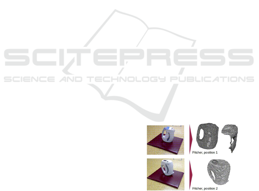
Figure 1: Example of a possible, and effortless, proce-

dure for acquisition of two non-overlapping meshes using

a Kinect sensor.

Another possible application of JASNOM is to ﬁll

holes in a mesh. In the case of interactive object mod-

eling, our algorithm allows a user to select parts from

a mesh or library of meshes and use them to ﬁll holes

in an incomplete 3D model. The possibility of ﬁll-

ing holes from other mesh parts is of valuable use for

modeling objects with self similar surfaces such as

planes or cylinders, which are the basic shapes of the

man-made objects that populate indoor environments.

JASNOM addresses jointly both the problem of

registration and merging of meshes by aligning two

meshes by their boundary. As depicted in Figure 2,

667

Brandão S., P. Costeira J. and Veloso M..

Effortless Scanning of 3D Object Models by Boundary Aligning and Stitching.

DOI: 10.5220/0004746406670674

In Proceedings of the 9th International Conference on Computer Vision Theory and Applications (VISAPP-2014), pages 667-674

ISBN: 978-989-758-003-1

 2014 SCITEPRESS (Science and Technology Publications, Lda.)

JASNOM aligns two meshes, M

and M

, and glues

them to create a single mesh, M. While JASNOM

applications can be extended to any problem that can

be formulated by boundary alignment, e.g., puzzles,

JASNOM was developed with a primary focus on 3D

object modeling.

Figure 2: Our objective is to construct a mesh M from two

other meshes, M

and M

. Both meshes have a boundary B

and B

that do not overlap. To construct M, we align both

boundaries through a rotation R and a translation

JASNOM aligns meshes by assuming that their

boundaries are the same geometric structure but seen

in different reference frames, i.e., that each point in

one boundary has a corresponding point in the other.

Under this assumption, stitching edges should con-

nect corresponding vertices in the two boundaries and

should have zero length. The stitching problem can

then be posed as that of ﬁnding correspondences be-

tween boundaries and the aligning problem as that of

ﬁnding the rigid transformation that minimizes the to-

tal edge length.

However, in a realistic scenario, the boundaries do

not exactly match and there is no a-priori knowledge

on the correspondences between the boundaries. In

this case, the previous solution would have three main

draw backs: i) if the boundaries are strongly irregu-

lar, simple minimization of edge lengths may lead to

intersections between meshes; ii) in general, ﬁnding

correspondences between vertices is a combinatorial

problem; iii) there is no guarantee that the correspon-

dences by themselves will deﬁne a a triangular mesh

that allows the completion of the mesh.

Our main contributions address these problems

and allow the reconstruction of a triangular mesh be-

tween the two boundaries. Namely JASNOM:

• introduces a cost function that penalizes both the

edge lengths and the intersection between meshes;

• introduces constraints that simplify the search for

the assignments from a combinatorial problem to

a discrete linear programming problem, solvable

in linear time;

• introduces a stitching algorithm that reconstructs

the triangular mesh given a set of assignments.

JASNOM penalizes the intersection between

meshes by modeling the intersection as a set of lo-

cal conditions to be veriﬁed by each stitching edge.

Section 3 introduces the cost function and our mini-

mization strategy.

To constrain the search space for the assignments,

JASNOM uses the fact that the resulting mesh should

have the same properties as an object surface. E.g.,

object surfaces are 2D-manifolds and thus object sur-

face meshes cannot have edges crossing each other

except at vertices. Section 4 addresses some prop-

erties of object surface meshes and their impact on

establishing assignments between boundaries.

To reconstruct the mesh structure, JASNOM

makes use of the assignments from the alignment

stage and ensures that properties like mesh manifold-

ness are locally preserved. Section 5 addresses the

problem of reconstructing meshes from assignments.

Section 6 illustrates different applications of JAS-

NOM and Section 7 concludes.

2 RELATED WORK

The use of range images for 3D object modeling moti-

vates the use of mesh stitching to construct complete

models. Due to their planar topology, range images

induce an intrinsic mesh in point clouds, but do not

represent the whole object. Thus, to recover the com-

plete object surface, several meshes from range im-

ages can be stitched together, instead of using point

cloud ﬁltering approaches, such as (Kazhdan et al.,

2006), (Levin, 2003), (Guennebaud and Gross, 2007)

or (Newcombe et al., 2011), or using approximations

to the convex-hull, such as (Edelsbrunner and M¨ucke,

1994) or ball pivoting (Bernardini et al., 1999). In

terms of applications, we note that using the original

mesh and vertices instead of using pos-processing ap-

proaches introduces several advantages, e.g., adding

color to the models is immediate. As such, we here

focus on other works that preserve the original mesh.

In (Turk and Levoy, 1994), authors present a three

step algorithm for stitching range images that makes

use of the overlap between images to both align and

stitch them. The algorithm ﬁrst step is to align meshes

by means of an Iterative Closest Point (ICP) algo-

rithm, (Besl and McKay, 1992). The second step

VISAPP2014-InternationalConferenceonComputerVisionTheoryandApplications

668

removes overlapping regions between two adjacent

meshes, by deleting triangles. This step leaves only

the triangles that do not overlap or that overlap only

partially. The ﬁnal step stitches meshes by the points

where the partially overlappedtriangles intersect. The

stitching procedure adds vertices at the intersection

and new triangles are built on top of the original ones.

When there is no overlap, meshes cannot be aligned

using ICP and the stitching cannot be built on top of

existing triangles.

More recently, different authors, e.g. in (Marras

et al., 2010) and (Pauly et al., 2005), used the tech-

nique described in (Turk and Levoy, 1994) for mesh

stitching with the purpose of ﬁlling holes in a model.

In both algorithms an initial step for mesh alignment

was required. However, while (Marras et al., 2010)

used parts of the same object from different meshes

to ﬁll in the holes, (Pauly et al., 2005) used parts of

other objects. Because the objects are different, in-

stead of aligning the meshes with an ICP type of al-

gorithm, (Pauly et al., 2005) resorts to non rigid de-

formations. Both algorithms used the stitching algo-

rithm proposed in (Turk and Levoy, 1994) to combine

different meshes.

Other approaches to the stitching itself, but that

assume that meshes were also previously registered

are presented in (Borodin et al., 2002) and (Soucy and

Laurendeau, 1995). The former algorithm stitches

by introducing new edges and minimizes their length

by creating and deleting vertices in the boundaries.

In our algorithm, JASNOM, we also focus on mini-

mizing the edge length, but we do it for the purpose

of ﬁnding a rigid transformation that aligns the two

meshes. The algorithm in (Soucy and Laurendeau,

1995) uses a Delaunay triangulation on a reprojection

of non-overlapping meshes. However, the complete

algorithm assumes that there is a very ﬁne alignment

between meshes.

JASNOM adds to the capabilities of the previous

algorithms, the possibility of aligning meshes with no

overlap and connecting meshes without resorting to

existing triangles to ensure manifoldness.

3 MESH ALIGNMENT

JASNOM addresses the problem of aligning and

stitching two meshes M

and M

by focusing on the

boundaries of each mesh, B

and B

as shown in Fig-

ure 3. In particular, JASNOM creates a complete

mesh by assigning new edges from one boundary to

the other and minimizing the total length of these

edges by means of a rigid transformation. Further-

more, while minimizing edge length, it must prevent

Rotation

Translation

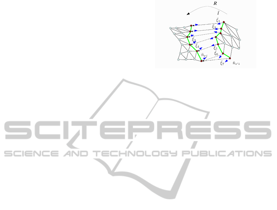
Figure 3: The two meshes are connected by assigning edges

from one boundary to the other. We represent edges by er-

ror vectors ξ

whose coordinates depend on R and

t. The

smaller vectors, ¯n

v,v

′

, correspond to the boundary normals

at the vertices.

the meshes from intersecting each other. Formally,

JASNOM solves an optimization problem whose cost

function, J, is composed of two independent terms J

and J

. The ﬁrst term, J

, penalizes the total edge

length, while J

penalizes the intersection. The result

of the optimization is the mesh alignment and a initial

set of assignments that will later be used for stitching.

3.1 Minimizing Edge Lengths

To ensure that edges are as small as possible, JAS-

NOM addresses the aligning of two meshes as a reg-

istration problem, where edges represent assignments

between vertices in the two meshes. These assign-

ments are represented by a binary matrix A, whose

element A

i, j

is equal to 1 if and only if vertex v

boundary B

is connected to vertex v

′

in boundary B

Assuming there are K vertices in B

and N vertices in

, A ∈ {0,1}

K×N

and if no additional constraints are

added, there are 2

K×N

different assignment matrices.

Matrix A deﬁnes a set of error vectors,

, each

associated to a stitching edge. The error vector rep-

resents the displacement between assigned vertices in

the two borders:



∑

j=1

i, j

¯x



− ¯y

′

, where ¯x

and ¯y

′

are the coordinates of the vectors in B

and

in the same reference frame. However we only

have access to the coordinates in the original refer-

ence frames, which differ by a rotation R and a trans-

lation

t. Therefore, the cost function J

, responsible

for minimizing the length of the stitching edges, is

given by Eq.1.

(A,R,

t) =

∑

i=1

∑

i=1



∑

j=1

i, j

¯x

− R¯y



(1)

EffortlessScanningof3DObjectModelsbyBoundaryAligningandStitching

669

3.2 Preventing Intersection

To globally ensure that no intersection occurred, JAS-

NOM would have to check for local intersections be-

tween each and all the vertices in one mesh versus

each and all the faces of the other mesh. JASNOM

relaxes the problem by considering only intersections

between a vertex v

′

∈ B

and the neighborhood of

∈ B

to which it was assigned.

Local intersections can be modeled by keeping

track of the position of mesh M

1,2

with respect to each

vertex of the boundary B

1,2

. This relative position is

represented for each boundary vertex v by the normal

to the boundary ¯n

, as shown in the Figure 3. Keeping

in mind that error vectors

ξ point from vertices v

′

∈ B

to vertices v ∈ B

, if

points in the opposite direction

of ¯n

′

, the vertex v

′

∈ B

is on top of mesh M

Ideally, preventing intersections would then result

on a set of constraints in the optimization problem.

However, since the estimation of the boundary nor-

mals is very sensible to noise and irregularities on the

boundary, the constraints may yield the problem un-

solvable. We thus relax these constraints by introduc-

ing them as a second term to the cost function, J

. The

constraints are modeled as a sum of logistic functions

that receive as argument the projection of

on − ¯n

and ¯n

′

as in Eq.2. The logistic function penalizes

edges that cross the opposite boundary by penalizing

the negative projections on ¯n

′

and the positive pro-

jections on ¯n

(A,R,

t,λ) =

∑

k=1

1/N

1+ exp{λ

· ¯n

′

∑

k=1

1/N

1+ exp{−λ

· ¯n

(2)

We introduce a slack variable λ to control the

steepness of the logistic function. High values of λ

correspond to steepest transitions on the logistic func-

tion and enforce the constraints more strictly. Lower

values of lambda relax the constraints. The best value

depends on the conﬁdence on the normal estimation.

3.3 Minimizing the Cost Function

Formally, JASNOM aligns and stitches the two

meshes by ﬁnding the matrices A and R and the vector

t that solve the optimization problem deﬁned in Eq. 3

J(A,R,

t;λ,ν) = J

(A,R,

t) + µJ

(A,R,

t, λ) (3)

s.t. A ∈ {0, 1}

N×K

, R ∈ O(3),

t ∈ R

;

where ν ∈ R

weights the two cost functions and de-

pends on the object or application. E.g., if the task is

hole ﬁlling and the patch we use is smaller than the

hole there will be no intersection and thus µ can be

set to zero.

Without further constraints, ﬁnding the matrix A

is a combinatorial problem. However, we note that if

the assignments between meshes correspond to edges

in the mesh of an object, not all the assignments are

valid. For example, no edge can cross the interior

of the object. We explore the physical constraints

in the problem to reduce the number of possible as-

signments between the two meshes. The constraints,

which we address in Section 4, are independent of the

rigid transformation that aligns the two meshes.

JASNOM is then able to tackle separatedly the

discrete problem of ﬁnding the assignment matrix A

from the problem of ﬁnding the rigid transformation,

R and

t. The separation and reduced complexity al-

low the algorithm to address the discrete problem by

enumeration, i.e., JASNOM minimizes J(A, R,

t) by

ﬁnding the minimum over the set of all valid assign-

ments, V

, using exhaustive search.

argmin

A,R,

J(A,R,

t) = argmin

J(R,

t;A

) (4)

s.t. A

∈ V

J(R,

t;A

) = min

J(A

,R,

t) (5)

The optimization problem expressed in Eq. 5 is

non-convex. To ﬁnd a local solution, we use a generic

non-linear optimization algorithm, such as BFGS

Quasi-Newton method (Broyden, 1970). To initial-

ize the optimization, JASNOM ﬁrst solves the relaxed

problem obtained from Eq. 3 by setting µ = 0, which

has a closed form solution (Sch¨onemann, 1966).

4 VALID ASSIGNMENTS

Stitching assignments in JASNOM correspond to

edges in an object surface and, as shown in Fig-

ure 4(a.2), these edges have a speciﬁc geometric

structure. In the following, we address the geomet-

ric properties that can be used to constrain possible

assignments and then present how JASNOM uses the

constraints to efﬁciently ﬁnd the best stitching edges.

4.1 Assignment Constraints

The complete surface mesh of an object is an ori-

entable 2-manifold mesh, while an isolated part of

the surface is an orientable 2-manifold mesh with a

boundary. In Figure 4(a.2) we exemplify the mesh

structure corresponding to an object part. In partic-

ular, we note that there are only two types of edges:

VISAPP2014-InternationalConferenceonComputerVisionTheoryandApplications

670

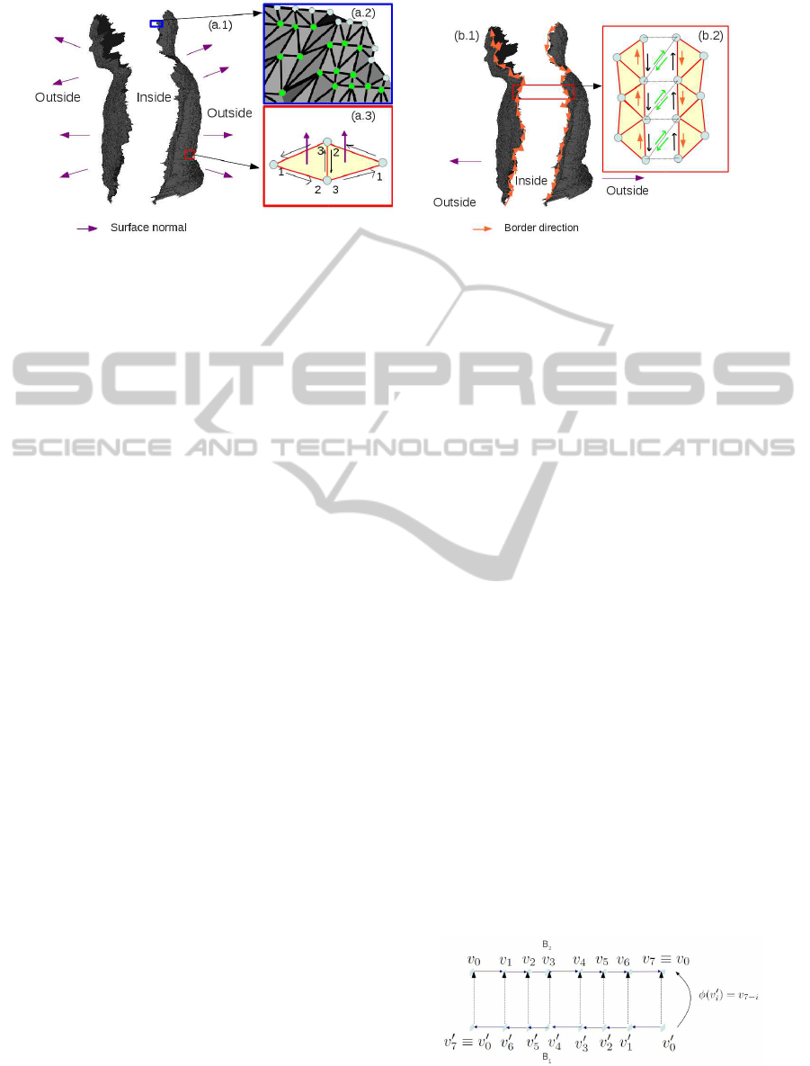
(a) Object surface orientability at global and local scale. (b) Orientation of boundary edges.

Figure 4: Order constraints on the boundary vertices. The image on the left shows how the orientability of an object induces

an ordering at the edge level. The image on the right shows how the ordering is reﬂected in the boundary and how does it

constraints the assignments between boundaries. See the text for further explanations.

those that belong to two triangles, and those that be-

long to only one, i.e., that are in the mesh boundary.

Formal deﬁnitions of all these concepts can be found

in computational geometry books, e.g., (Munkres,

1984). We brieﬂy illustrate them here to allow a better

comprehension of the constraints.

Object surfaces are orientable because they have

an inside and an outside. Using one of these direc-

tions, it is possible to deﬁne consistently the normal

directions for all points at the surface as shown in

Figure 4(a). For 2-manifold meshes, the deﬁnition

of a normal to a triangle is associated with a cyclic

order of the triangle vertices. The normal to a tri-

angle with vertices v

, v

and v

with coordinates

¯x

, ¯x

∈ R

can be estimated by the outer product

ˆn

= ( ¯x

− ¯x

) × (¯x

− ¯x

). If the order of the vertices

changes, the direction of the normal vector will be the

exact opposite. To ensure consistency on the orien-

tation of two adjacent faces, the two vertices of the

common edge must be in opposite order, as shown in

Figure 4(a.3). Boundary edges have only one possi-

ble orientation since they belong to a single triangle.

This orientation deﬁnes the intrinsic direction of the

boundary cycle, as shown in Figure 4(b).

The whole surface mesh is orientable if all adja-

cent faces are consistent. To guarantee that the union

of two meshes is orientable, their boundaries cannot

have a random orientation with respect to each other.

JASNOM stitches two meshes by assigning an edge

from one boundary to the other. This situation, illus-

trated in Figure 4(b.2), requires the orientation of the

boundaries to oppose each other. This is in consis-

tency with the Gluing theorem.

Since the union of the two meshes is introduced

by the assignment matrix A, the matrix must reﬂect

the ordering of the two boundaries. We thus introduce

the constraint: A

i, j

= 1 ⇒ A

i+1, j+k

= 0, ∀k ≥ 0.

4.2 Order Preserving Assignments

The space of matrices that satisfy the previous con-

straint is still very large. To further constrain the

valid assignments search space, V

, we introduce

some geometric constraints. In particular, we note

that if the two meshes were the exact complemen-

tary of each other over the object surface, the two

boundaries would correspond to the same vertices and

edges. In this case, given a mapping φ : B

→ B

between the two boundaries that returns the point

∈ B

equivalent to the point v

′

∈ B

, we can de-

ﬁne the assignment between the two boundaries as

i, j

= 1 ⇔ v

= φ(v

′

To construct this mapping, we deﬁne one origin

in each boundary, and order the vertices according to

the boundary orientation. Assuming that the origins

correspond to the same point, two points that are at the

same distance, i, from the origin, should be equivalent

to each other. To account for the opposite boundary

orientations, the mapping needs to invert the vertex

ordering, e.g., as in φ(v

′

) = v

N−i

. This is illustrated in

Figure 5 where N refers to the total number of vertices

in the boundary and i to the order of the vertex v

′

with

respect to the boundary of B

For the vertices of the two boundaries to map to

each other, the sampling in both surfaces has to be

exactly the same. Thus, in most cases, mapping the

Figure 5: Example for the construction of an assignment

between boundaries in the limit case where the vertices in

both boundaries coincide exactly.

EffortlessScanningof3DObjectModelsbyBoundaryAligningandStitching

671

vertices order across boundaries does not preserve the

object geometry. It is then more reasonable to map

distances over the boundaries. In this work, we use

the normalized curve length l ∈ [0,1] to account for

those cases when the boundaries do not have the exact

same length. In this case, the previous map can be

rewritten as ϕ(l

′

) = 1− l.

After mapping a point between boundaries based

on the normalized length, JASNOM still needs to ﬁnd

the closest vertexto that point. This search can be efﬁ-

ciently implemented by introducing an ordering func-

tion f(l) : [0,1] → [0,N], which maps lengths over a

speciﬁc boundary to a vertex order. For example, if

vertex v

is at a length l

, f(l

) = k. For values of l

that do not correspond to exact vertices length but to

points on the boundary edges, f(l) returns the order

of the closest vertex.

Using the map ϕ(l

′

) and knowing the ordering

function f(l) for B

, we can ﬁnd the order j of the

vertex v

∈ B

to which assign v

′

∈ B

by performing

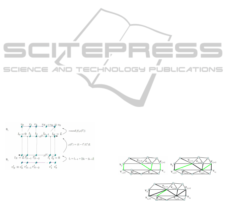
three steps. Namely:

i) computing the length l

′

= l

′

) = l

′

i−1

k ¯y

− ¯y

i−1

ii) mapping the length l

′

to the length l of the equiv-

alent point in B

: l = ϕ(l

′

));

iii) ﬁnding the vertices in B

that have a distance to

the boundary closest to l using the ordering func-

tion over B

: j = f(ϕ(l

′

))).

The three steps are illustrated in Figure 6.

Figure 6: Three steps approach to deﬁne order preserving

assignments between the boundaries. See text for details.

By repeating for all v

∈ B

, JASNOM deﬁnes the

assignment matrix A as

i, j

= 1 ⇔ j = round( f(ϕ(l

′

)))) (6)

The previous deﬁnition for A depends only on the

map ϕ and the ordering function f(l). However, both

functions depend on the vertex deﬁned as an origin

on either boundary. If any other vertex v

′

∈ B

was

assumed to be equivalent to the origin, v

∈ B

, the

mapping could be recovered by shifting l

′

by l

. This

origin ambiguity is translated into N different valid

maps between boundaries.

JASNOM addresses the ambiguity problem by

considering all possible N different shifts τ of the

boundary B

with respect to the boundary B

. Each

shift gives rise to a new mapping ϕ

and each map-

ping gives rise to a new assignment matrix A

. Thus,

the combinatorial problem can be reduced into N in-

dependent problems. We note that by changing the

shift in B

and not in B

, the ordering function de-

ﬁned in B

will be the same in all the shifts in A

5 FINAL STITCHING

After aligning both meshes, JASNOM uses the best

assignment to reconstruct the manifold M

. In partic-

ular, the assignment as deﬁned in 6 ensures that each

vertices in B

already has an edge connecting it to a

vertex in B

. However, not all the vertices in B

have

an edge connecting to B

and some vertices in B

have

more than one edge. Furthermore, just ensuring that

there is an edge for all the vertices, does not ensure

that the end result is a triangular mesh.

To stitch the meshes together, we use two simple

strategies. First, we create a triangular mesh from

the assignments already present. Then we assign the

missing edges on B

so that they do not cross the

edges already present.

For the ﬁrst step, JASNOM adds a second edge to

all the vertices v

′

∈ B

. As shown in Figure 7(b), the

target vertex, v

∈ B

of the second edge of v

′

is the

the ﬁrst target of the next vertex, v

′

i+1

∈ B

In the second step JASNOM assigns the missing

edges in B

by running through all the vertices v

∈ B

by their reverse order. As shown in Figure 7(c) each

vertex with no edge is assigned the same target vertex

′

∈ B

as the target of the previous vertex v

j−1

∈ B

(a) Best assignment (b) Second edge to B

Figure 7: Schematic for the stitching between the two

meshes given the set of one to one correspondences that

result from the alignment stage. See the text for comments.

This strategy locally ensures manifoldness since

there are no crossings between neighboring edges.

The constraints in the assignments ensure that the ini-

tial set of edges do not cross and the newedges always

preserve the ordering between boundaries.

VISAPP2014-InternationalConferenceonComputerVisionTheoryandApplications

672

In summary, JASNOM creates a complete 3D ob-

ject surface model from non overlapping meshes by

enumerating all valid assignment matrices, A

∈ V

and, for each matrix, ﬁnding the rigid transformation

that minimizes the cost function J(A

,R,

t). JASNOM

chooses the best assignment as the one that mini-

mizes the cost function over all the minima, and aligns

the meshes accordingly. This assignment serves also

as initialization to the stitching algorithm, where the

missing triangles are added.

6 PROOF OF CONCEPT

We test our stitching algorithm with three experi-

ments. In the ﬁrst we illustrate its potential for fast 3D

object scanning by modeling two smooth objects. In

the second, we illustrate its potential for reconstruct-

ing 3D models from articulated objects such as hu-

mans. Finally, in the third experiment, we illustrate

its potential for hole ﬁlling.

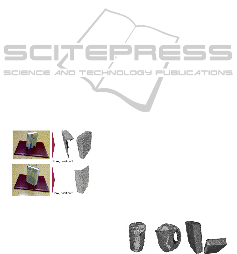
For the ﬁrst experiment, we model two objects.

The ﬁrst is the electric pitcher, Figure 1, and the sec-

ond a book, Figure 8. To collect both meshes for the

example, we retrieve an image with the object in its

regular position and then ﬂip it upside down to collect

the second image. The complete process is extremely

fast from a user perspective and does not require pre-

vious registration of multiple cameras. The resulting

complete meshes are presented in Figure 9.

Figure 8: Acquisition of two meshes from a book.

For the purpose of accuracy while estimating cen-

troids and other intermediate steps, JASNOM interpo-

lates boundaries to ensure an uniform and dense dis-

tribution of points. To deal with the non-compactness

of the object, JASNOM selected just the longest

boundary. We note that the reconstructed objects

show a good match at the boundaries.

For the second experiment, two range images of

the upper body of a human were retrieved simulta-

neously by two unregistered Kinect cameras. The

complete mesh obtained with JASNOM algorithm is

shown in Figure 10. We note that the two meshes do

not cover the complete object and there are several

large missing parts across the boundary. However, by

preventing intersection, JASNOM was able to keep

the overall human structure. In particular, the hole

created by the cut at the waist is large enough that by

simply attempting to minimize the distance between

points, would lead to mesh intersections. Again we

note that, with no previous camera registration, JAS-

NOM created a rough shape of a non-rigid object us-

ing two Kinect cameras.

For the last experiment, we use a simple range im-

age of an object with a hole and a small patch re-

trieved from another mesh, Figure 11(a). JASNOM

covered and stitched the hole, Figure 11(b). Since

the objective is to insert the patch on the hole in the

other mesh, we did not penalize intersections between

meshes, i.e., µ = 0. We note that in this case the

re-triangulation method left a smooth surface after

patching the hole.

7 CONCLUSIONS

In this work we have contributed an algorithm, JAS-

NOM, that allows the joint alignment and stitching of

non-overlappingmeshes, and provided evidence of its

potential for fast 3D object scanning through simple

experiments with data obtained with a Kinect camera.

From the experiments we conclude that JASNOM

successfully constructs 3D models of different object

types, including rigid and non rigid. The success of

JASNOM is due mostly to the cost function deﬁni-

tion. By preventing the intersection between bound-

aries, JASNOM preserves the object structure even

with noisy boundaries. JASNOM is thus able to re-

construct complex shapes with missing parts such as

the human we presented.

When compared with existing stitching algo-

rithms, JASNOM adds the capability to create com-

plete models without previous registration of individ-

ual meshes. The registration typically requires over-

lap between the two meshes, which is not always

available or convenient. JASNOM also does not re-

Figure 9: Reconstruction of man made objects using JAS-

NOM. The ﬁrst row presents two different views from the

electric pitcher and the second from the book.

EffortlessScanningof3DObjectModelsbyBoundaryAligningandStitching

673

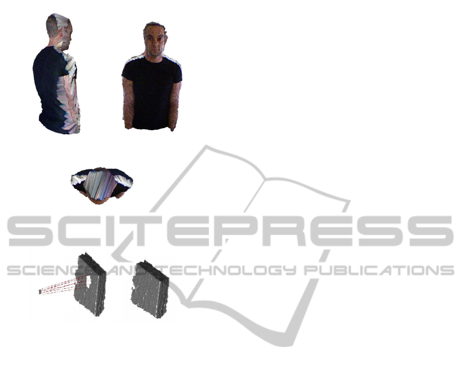
(a) Back (b) Front

Figure 10: Human model completed using JASNOM.

(a) (b) Hole ﬁlled.

Figure 11: Results for the hole patching experiment using

JASNOM. Figure 11(a) presents the original mesh with a

hole and the patch. Figure 11(b) presents the glued mesh.

quire the calibration of one camera position with re-

spect to the other. The registration and construction

of models can be easily achieved with little effort and

setup preparation. This allows for the fast creation of

extensive 3D (possibly 3D+RGB) models data sets.

JASNOM assumes that the two meshes are com-

plementary over the object surface and, while we

showed it could reconstruct objects in more general

cases, e.g., the human shape, other objects might not

be reconstructed so easily. In particular, we note that

the boundaries of the human shape meshes, had a

preferential direction, i.e., the elongated shape means

that small deviations from the best assignment be-

tween boundaries lead to steep increases in the cost

functions. More symmetric objects do not beneﬁt

from the steepness in the cost function and the align-

ment is more sensitive to gaps between boundaries.

A possible approach, which we will explore in future

work, is to reintroduce the asymmetries by penalizing

color discontinuities at the boundaries.

ACKNOWLEDGEMENTS

This research was partially sponsored by the

Portuguese Foundation for Science and Technol-

ogy through both the CMU-Portugal and PEst-

OE/EEI/LA0009/2013 project, and the National Sci-

ence Foundation under award number NSF IIS-

1012733, and the Project Bewave-ADI. Jo˜ao P.

Costeira is partially funded by the EU through ”Pro-

grama Operacional de Lisboa”. The views and con-

clusions expressed are those of the authors only.

REFERENCES

Bernardini, F., Mittleman, J., Rushmeier, H., Silva, C., and

Taubin, G. (1999). The ball-pivoting algorithm for

surface reconstruction. Trans. VCG.

Besl, P. J. and McKay, N. D. (1992). A method for registra-

tion of 3-d shapes. PAMI, 14(2):239–256.

Borodin, P., Novotni, M., and Klein, R. (2002). Progres-

sive gap closing for mesh repairing. In Vince, J. and

Earnshaw, R., editors, Adv. in Mod. Anim. and Rend.

Broyden, C. G. (1970). The convergence of a class of

double-rank minimization algorithms. JIMA.

Edelsbrunner, H. and M¨ucke, E. P. (1994). Three-

dimensional alpha shapes. Trans. Graph., 13(1).

Guennebaud, G. and Gross, M. (2007). Algebraic point set

surfaces. ACM Trans. Graph., 26(3).

Kazhdan, M., Bolitho, M., and Hoppe, H. (2006). Poisson

surface reconstruction. In Eurographics.

Levin, D. (2003). Mesh-independent surface interpolation.

Geometric Modeling for Scientiﬁc Visualization, 3.

Marras, S., Ganovelli, F., Cignoni, P., Scateni, R., and

Scopigno, R. (2010). Controlled and adaptive mesh

zippering. Comp. Graphics Theory and Applications.

Munkres, J. (1984). Elements of Algebraic Topology. West-

view Press.

Newcombe, R. A., Izadi, S., Hilliges, O., Molyneaux, D.,

Kim, D., Davison, A. J., Kohli, P., Shotton, J., Hodges,

S., and Fitzgibbon, A. (2011). Kinectfusion: Real-

time dense surface mapping and tracking. In ISMAR.

Pauly, M., Mitra, N. J., Giesen, J., Gross, M., and Guibas,

L. (2005). Example-based 3d scan completion. In

Symposium on Geometry Processing.

Sch¨onemann, P. (1966). A generalized solution of the or-

thogonal procrustes problem. Psychometrika.

Soucy, M. and Laurendeau, D. (1995). A general surface

approach to the integration of a set of range views.

PAMI, 17(4):344–358.

Turk, G. and Levoy, M. (1994). Zippered polygon meshes

from range images. In SIGGRAPH.

VISAPP2014-InternationalConferenceonComputerVisionTheoryandApplications

674