Fast Optimum-Path Forest Classiﬁcation on Graphics Processors

Marcos V. T. Romero

, Adriana S. Iwashita

, Luciene P. Papa

, Andr´e N. Souza

and Jo˜ao P. Papa

Department of Computing, S˜ao Paulo State University, Bauru, S˜ao Paulo, Brazil

Southwest Paulista College, Avar´e, S˜ao Paulo, Brazil

Department of Electrical Engineering, S˜ao Paulo State University, Bauru, S˜ao Paulo, Brazil

Keywords:

Optimum-Path Forest, Graphics Processing Unit.

Abstract:

Some pattern recognition techniques may present a high computational cost for learning samples’ behaviour.

The Optimum-Path Forest (OPF) classiﬁer has been recently developed in order to overcome such drawbacks.

Although it can achieve faster training steps when compared to some state-of-art techniques, OPF can be

slower for testing in some situations. Therefore, we propose in this paper an implementation in graphics cards

of the OPF classiﬁcation, which showed to be more efﬁcient than traditional OPF with similar accuracies.

1 INTRODUCTION

Pattern recognition techniques have as main goal to

classify a dataset based on a previous learning over

some predeﬁned samples, which are described by

a set of features extracted from an observation set,

deﬁning points on a multidimensional space. De-

pending on the information we have about the dataset,

we can face unsupervised and supervised techniques,

where a fully labeled dataset can enhance the effec-

tiveness of such approaches (Duda et al., 2000).

Supervised learning approaches allow the classi-

ﬁer to learn the behaviour of the dataset from a train-

ing set, and then evaluate this learning applying the

knowledge over an unseen test set. Recently, a graph-

based framework for supervised pattern recognition

techniques was proposed by Papa et al. (Papa et al.,

2009; Papa et al., 2012). The Optimum-Path Forest

(OPF) classiﬁer models pattern recognition as an opti-

mum graph partition problem, in which a competition

process among some samples generates a collection

of optimum-path trees (OPTs) rooted at them. Each

class can be represented by just one or several OPTs,

which encode the power of connectivitybetween sam-

ples.

Even though OPF has obtained results compara-

ble to the ones given by some state-of-the-art pat-

tern recognition techniques, such as Support Vector

Machines (SVM) and Neural Networks (NN), being

also faster than them for training, the OPF classiﬁca-

tion has a considerable computational burden. While

SVM testing phase uses only the support vectors com-

puted in the training phase, and for NN we need only

the neurons’ weights, in regard to OPF it is required

to compute the distance for all training set to classify

just one test sample. Although Papa et al. (Papa et al.,

2012) have proposed an optimization of this step, the

OPF test phase may be still time consuming.

Aiming to achieve even faster classiﬁcation

phases, some works have presented implementations

of pattern recognition techniques in CUDA (Compute

Uniﬁed Device Architecture) environment, which

makes use of the high number of cores embedded

on the Graphic Processing Unit (GPU) of some re-

cent graphics cads. Catanzaro et al. (Catanzaro et al.,

2008), for instance, proposed a GPU-based imple-

mentation of SVM which is around 9 −−35× faster

than traditional implementation on CPU (Central Pro-

cessing Unit). Oh and Jung (Oh and Jung, 2004) have

introduced neural networks in the context of GPU-

based programming.

Further, Jang et al. (Jang et al., 2008) proposed

a NN implementation combining CUDA e OpenMP

(Open Multi-Processing). In this work, the authors

argued about the massive parallel programming in

GPUs, in which we need to take care about the gran-

ularity of the problem. Therefore, the amount of

source code which can be parallelized must counter-

balance the system’s throughput. Recently, Gainaru

et al. (Gainaru et al., 2011) presented a study about

some data mining algorithms implemented on GPU

devices.

In this work, we present a CUDA-based OPF test-

ing phase, as well as some experiments which shown

627

V. T. Romero M., S. Iwashita A., P. Papa L., N. Souza A. and P. Papa J..

Fast Optimum-Path Forest Classiﬁcation on Graphics Processors.

DOI: 10.5220/0004740406270631

In Proceedings of the 9th International Conference on Computer Vision Theory and Applications (VISAPP-2014), pages 627-631

ISBN: 978-989-758-004-8

 2014 SCITEPRESS (Science and Technology Publications, Lda.)

the gain on efﬁciency keeping similar recognition

rates when compared with traditional OPF. As far as

we know, this is the ﬁrst proposal of one GPU-based

implementation of OPF up to date. The remainder of

this paper is organized as follows. Section 2 and 3

present OPF background and the approach approach

to boost OPF testing step. Section 4 discusses the ex-

perimental results and Section 5 states conclusions.

2 OPTIMUM-PATH FOREST

Let X and Y be a set of samples and their correspond-

ing labels, respectively, where Y ⊆ M , being M the

set of all possible labels. Given a labeled dataset

D = (X , Y ) , the idea behind OPF is to model D as

a graph G = (V , A) whose nodes are the samples in

V = X , and the arcs are deﬁned by an adjacency re-

lation A between nodes in the feature space. The arcs

are weighted by a distance function between the fea-

ture vectors of the corresponding nodes.

As a community ordered formation process,

where groups of individuals are obtained based on

optimum connectivity relations to their leaders, OPF

employs a competition process among some key

nodes (prototypes) in order to partition the graph into

an optimum-path forest according to some path-cost

function. By analogy, the population is divided into

communities, where each individual belongs to the

group which offered to it the highest reward. In ad-

dition, the dataset D is divided in two subsets D =

∪D

, standing for the training and test sets, re-

spectively. Now, we have the following graphs: G

, A

) and G

= (V

, A

), V

∪V

= X , which

model D

and D

, respectively.

Now assume π

be a path in the graph with termi-

nus at sample s ∈ D

, and hπ

·(s, t)i a concatenation

between π

and the arc (s, t). Let S ⊂ D

be a set

of prototypes from all classes. Roughly speaking, the

main idea of the Optimum-Path Forest algorithm is to

minimize a cost map O(t) = min

∀t∈V

{Ψ(π

)}, where

Ψ is a path-cost function deﬁned as:

Ψ(hsi) =



0 if s ∈S

+∞ otherwise,

Ψ(π

·hs, ti) = max{Ψ(π

), d(s, t)}, (1)

in which d(s, t) stands for the distance between nodes

s and t.

Particularly, an optimalset of prototypes S

∗

can be

found by exploiting the theoretical relation between

the minimum-spanning tree (MST) (Cormen et al.,

2001) and optimum-path tree for Ψ (All`ene et al.,

2007). By computing a MST in the complete graph

, we obtain a connected acyclic graph whose nodes

are all samples in V

. This spanning tree is optimum

in the sense that the sum of its arc weights is mini-

mum as compared to any other spanning tree in the

complete graph. In addition, every pair of samples

is connected by a single path, which is optimum ac-

cording to Ψ. Therefore, the optimum prototypes are

deﬁned as the nodes from distinct classes that share

an arc in the MST.

In the classiﬁcation phase, for any sample t ∈ V

we consider all arcs connectingt with samples s ∈V

as though t were part of the graph. Considering all

possible paths from S

∗

to t, we ﬁnd the optimum path

∗

(t) from S

∗

and label t with the class λ(R (t)) of

its most strongly connected prototype R (t) ∈ S

∗

, be-

ing λ(·) a function that returns the true label of some

sample. This path can be identiﬁed by evaluating the

optimum cost O(t) as:

O(t) = min{max{O(s), d(s, t)}}, ∀s ∈ V

. (2)

Suppose the node s

∗

∈ G

is the one which satis-

ﬁes (Equation 2). Given that label θ(s

∗

) = λ(R (t)),

the classiﬁcation simply assigns θ(s

∗

) as the class of

t. Clearly, an error occurs when θ(s

∗

) 6= λ(t), where

θ(·) stands for the predicted label for some sample.

3 PROPOSED ARCHITECTURE

FOR GPU-BASED OPF

In this section, we present the GPU-based implemen-

tation for OPF testing phase, as well as some deﬁ-

nitions employed in this work, which have been also

proposed to fulﬁll the development of the parallel ver-

sion of OPF.

3.1 Matrix Association

Let T be a matrix association operation between two

matrices A and B with dimensions n

×m and m×n

respectively. As a result of T, we can obtain a matrix

C with dimensions n

×n

, as follows:

C = T(A, B, f(x, y)), (3)

in which f(x, y) stands for a generic function, being

each element c

from C deﬁned as

∑

k=1

f(a

, b

), (4)

where a

and b

stand for elements from A and B,

respectively.

In order to make it clear, a matrix multiplication,

for instance, can be written as C = T(A, B, f(x, y)),

where f(x, y) is deﬁned as follows:

f(x, y) = x∗y. (5)

VISAPP2014-InternationalConferenceonComputerVisionTheoryandApplications

628

3.2 Parallel OPF Classiﬁcation on GPU

Devices

The main performance issue of the OPF testing phase

concerns with the distance calculation between all

training nodes and the testing sample. Such process is

used to ﬁnd the lowest path-cost given by some train-

ing node. Therefore, we propose here to parallelize

two steps of the OPF testing phase : (i) distance cal-

culation between training and testing nodes, and (ii)

ﬁnding the lowest path-cost given by some training

node to each testing sample.

In regard to the former step, suppose the testing set

can be modeled by a matrix M

with dimensions n

, in which n

and n

stand for the testing set size

and the number of features, respectively. Thus, each

rowi of M

represents the features from testing node i.

Similarly, the training set is then modeled by a matrix

with dimensions n

×n

, in which n

denotes the

training set size.

Assuming the Euclidean distance as the similarity

function (as employed the default distance by OPF),

the distance calculation step can be modeled as a ma-

trix association between M

(test set) and M

(training

set), being f(x, y) in Equation 3 given by:

f(x,y) = (x−y)

. (6)

Therefore, Equation 3 can be rewritten as follows:

C = T(M

, M

, f(x, y)). (7)

After that, a square root must be applied to each ele-

ment c

of the resulting matrix C in order to complete

the Euclidean distance computation:

←

√

. (8)

In order to address the second step of OPF classi-

ﬁcation phase, i.e., to ﬁnd the lowest path-cost given

by some training node to each test sample, it is ﬁrst

necessary to compute equation below:

← max{c

, cost

}, (9)

where cost

contains the optimum cost of the train-

ing node j, which is computed in the training step via

traditional OPF. Finally, c

contains all path-costs of-

fered to test sample i by training node j.

In order to solve Equation 2 for testing node i, we

just need to ﬁnd the lowest value in line i of matrix

C, which can be done in parallel with a reduction op-

eration. For such purpose, we have used a tree-based

parallel reduction operation (Harris, 2010).

4 EXPERIMENTAL RESULTS

In this section we present the experimental results

conducted to show the robustness of the proposed ap-

proach. We have designed two different scenarios for

performance comparisons using computers with dis-

tinct conﬁgurations: GPU 1 and GPU 2. The former

is equipped with an Intel Core 2 Quad Q9300 pro-

cessor with 3.24GHz, 4GB DDR3 1333MHz RAM

and an EVGA GeForce GTX 550 Ti 1GB GDDR5

video card with 192 CUDA cores. GPU 2 is equipped

with an Intel Core i7 3770 processor with 3.4GHz,

8GB DDR3 1600MHz RAM and a Gigabyte Geforce

GTX 680 2GB GDDR5 with 1536 CUDA cores. Ba-

sically, the ﬁrst conﬁguration is a low-cost computer

equipped with a not too old video card. On the other

hand, GPU 2 has been equipped with one of the best

Intel processors available on the market for domestic

users, and also one of the best single GPU video card

for domestic use.

Additionally, two distinct CPU-based equipments

have been used: CPU 1 and CPU 2, which have the

same conﬁgurations of GPU 1 and GPU 2, respec-

tively. The difference is that we did not employ the

graphics cards, since they have ran traditional OPF.

In regard to the operational system, we have used

Ubuntu Linux 12.04.1 x86

64 LTS for both scenarios.

We have used datasets with different number of

samples and features in order to evaluate the robust-

ness of GPU-based OPF classiﬁcation step. Database

1 and 2 refer to non-technical losses identiﬁcation

in power distribution systems and automatic Ptery-

gium recognition tasks, respectively, being private

datasets. Databases 3 and 4 concern with two pub-

lic available hyperspectral remote sensing images: In-

dian Pines (Landgrebe, 2005) and Salinas (Kaewpijit

et al., 2003). In this case, each pixel is described by

the brightness of each spectral band. Table 1 shows

the information about datasets.

Table 1: Description of the datasets.

Database

# of nodes # of features

Database 1 4952 8

Database 2 15302 89

Database 3 21025 220

Database 4

111104 204

In regard to the experiments, the datasets were

partitioned in two parts: one for training and another

one for testing phase. We used different set sizes in

order to plot a curve of performance, starting from a

training set with 10% of the original dataset and in-

creasing it until 90% with a 10% step. The remaining

dataset on each step has been used as the testing set.

For each step size, the experiments were executed 10

FastOptimum-PathForestClassificationonGraphicsProcessors

629

(a) (b)

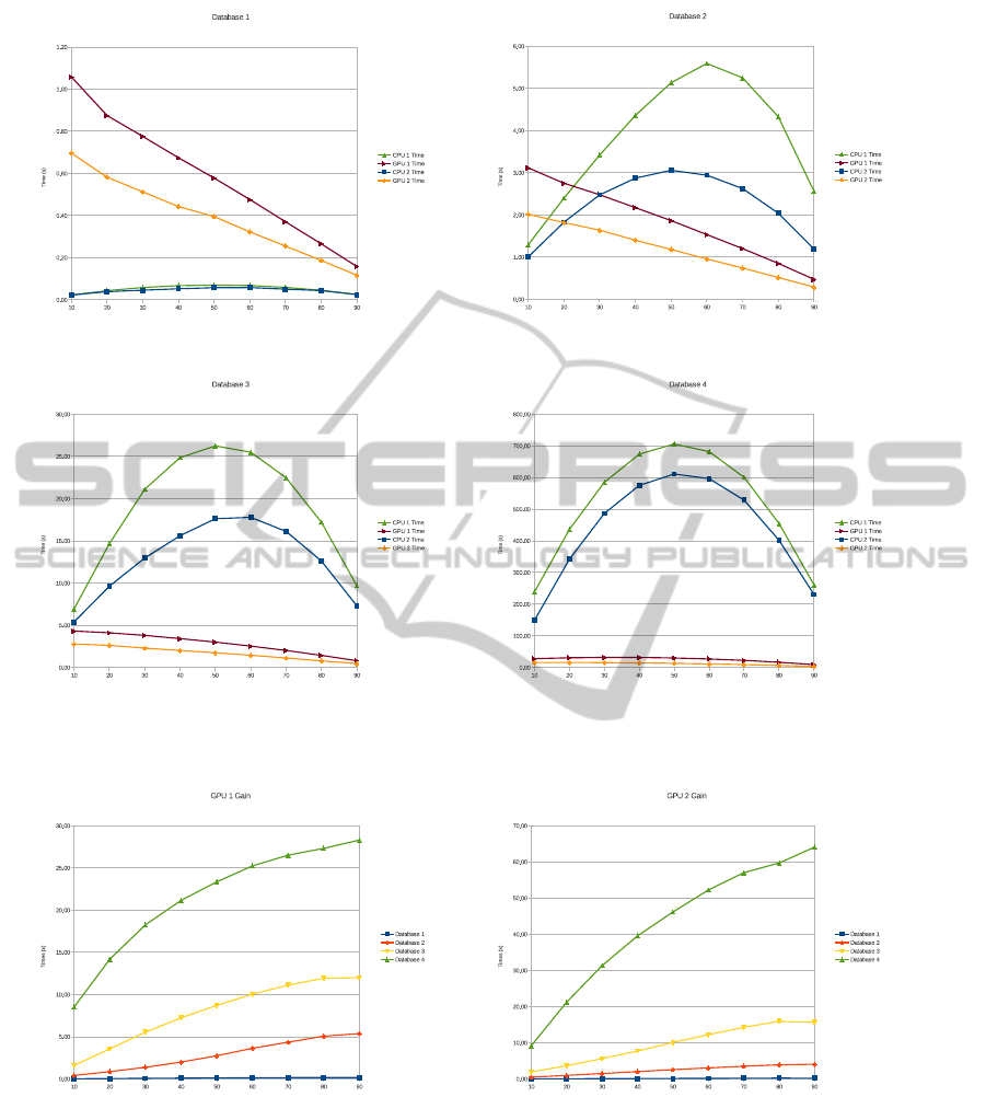
Figure 1: Performance curve for (a) Database 1, (b) Database 2, (c) Database 3 and (d) Database 4.

(a) (b)

Figure 2: Performance gain for (a) GPU 1 and (b) GPU 2.

times with training and testing sets randomly gener-

ated (cross-validation). Figure 1 displays the perfor-

mance curve for all datasets. Tables 2 and 3 display

the mean accuracy and execution times (seconds) for

Computer 1 and 2, respectively.

The reader can note GPU 2 has outperformed

GPU 1 and both CPUs for Databases 2, 3 and 4.

For Database 1, the trade-off between GPU gain and

throughput makes it inviable to the proposed algo-

rithm, since Database 1 is not large enough. In regard

to Database 2, the GPU gain can be observed at 20%

of training set size. Figure 2 presents the gain results

of the proposedapproach for both scenarios, i.e., GPU

1 and GPU 2. One can see it is possible to achieve

VISAPP2014-InternationalConferenceonComputerVisionTheoryandApplications

630

Table 2: Mean accuracy and execution times (s) for Com-

puter 1.

Data

Database 1 Database 2 Database 3

CPU Time 5.79 ± 0.29 26.13 ± 0.61 715.63 ± 4.31

CPU Acc. 56.07 ± 0.65 70.91 ± 0.73 90.98 ± 0.12

GPU Time

1.91 ± 0.05 3.05 ± 0.04 30.56 ± 0.33

GPU Acc. 55.97 ± 0.63 70.91 ± 0.73 90.99 ± 0.12

GPU Gain 3.03x 8.57x 23.42x

Table 3: Mean accuracy and execution times (s) for Com-

puter 2.

Data

Database 1 Database 2 Database 3

CPU Time 3.03 ± 0.03 17.46 ± 0.12 613.30 ± 2.74

CPU Acc. 56.02 ± 0.77 70.92 ± 0.62 91.08 ± 0.10

GPU Time

1.18 ± 0.01 1.75 ± 0.01 13.19 ± 0.04

GPU Acc. 56.00 ± 0.79 70.92 ± 0.62 91.08 ± 0.10

GPU Gain 2.57x 9.98x 46.50x

very interesting results with the proposed approach,

which can be better observed in large datasets.

5 CONCLUSIONS

This work presented a massive parallel approach for

OPF testing phase, A parallel operation called ma-

trix association, which can be seen as a generalization

of a matrix multiplication procedure, has been pro-

posed to consider this kind of data structure in order

to maximize the gain of GPUs. Experimental results

have shown the performance gain of the proposed ap-

proach in 3 out 4 databases, being the worst result in

the smaller database, which highlights the main usage

of GPU-based algorithms in applications that require

a large volume data.

It is worthy noting that GPU 1 conﬁguration can

be found at $130 by the time this article was submit-

ted, meaning that to develop parallel pattern recogni-

tion application is not exclusive only for those with

expensive equipments, even with large datasets.

ACKNOWLEDGEMENTS

The authors are grateful to FAPESP grants

#2009/16206-1, #2010/12697-8 and #2011/08348-

0, and CNPq grants #470571/2013-6 and

#303182/2011-3.

REFERENCES

All`ene, C., Audibert, J. Y., Couprie, M., Cousty, J., and

Keriven, R. (2007). Some links between min-cuts,

optimal spanning forests and watersheds. In Proceed-

ings of the International Symposium on Mathematical

Morphology, pages 253–264. MCT/INPE.

Catanzaro, B., Sundaram, N., and Keutzer, K. (2008). Fast

support vector machine training and classiﬁcation on

graphics processors. In Proceedings of the 25th inter-

national conference on Machine learning, pages 104–

111, New York, NY, USA. ACM.

Cormen, T. H., Leiserson, C. E., Rivest, R. L., and Stein, C.

(2001). Introduction to Algorithms. The MIT Press, 2

edition.

Duda, R. O., Hart, P. E., and Stork, D. G. (2000). Pattern

Classiﬁcation (2nd Edition). Wiley-Interscience.

Gainaru, A., Slusanschi, E., and Trausan-Matu, S. (2011).

Mapping data mining algorithms on a GPU architec-

ture: a study. In Proceedings of the 19th interna-

tional conference on Foundations of intelligent sys-

tems, ISMIS’11, pages 102–112, Berlin, Heidelberg.

Springer-Verlag.

Harris, M. (2010). Optimizing parallel reduction in CUDA.

Jang, H., Park, A., and Jung, K. (2008). Neural network im-

plementation using CUDA and OpenMP. In DICTA

’08: Proceedings of the 2008 Digital Image Com-

puting: Techniques and Applications, pages 155–161,

Washington, DC, USA. IEEE Computer Society.

Kaewpijit, S., Moigne, J., and El-Ghazawi, T. (2003).

Automatic reduction of hyperspectral imagery using

wavelet spectral analysis. IEEE Transactions on Geo-

science and Remote Sensing, 41(4):863–871.

Landgrebe, D. (2005). Signal Theory Methods in Multi-

spectral Remote Sensing. Wiley, Newark, NJ.

Oh, K. and Jung, K. (2004). GPU implementation of neural

networks. Pattern Recognition, 37(6):1311–1314.

Papa, J. P., Falc˜ao, A. X., Albuquerque, V. H. C., and

Tavares, J. M. R. S. (2012). Efﬁcient supervised

optimum-path forest classiﬁcation for large datasets.

Pattern Recognition, 45(1):512–520.

Papa, J. P., Falc˜ao, A. X., and Suzuki, C. T. N. (2009). Su-

pervised pattern classiﬁcation based on optimum-path

forest. International Journal of Imaging Systems and

Technology, 19(2):120–131.

FastOptimum-PathForestClassificationonGraphicsProcessors

631