Design of an Unstructured and Free Geo-Coordinates Information
Brokerage System for Sensor Networks using Directional Random Walks
Cristina Mu
˜
noz and Pierre Leone
Computer Science Department, University of Geneva, Carouge, Switzerland
Keywords:
Directional Random Walk, Information Brokerage, Unstructured Networks, Sensor Networks.
Abstract:
The main problem studied in this paper is how to design an efficient method for information brokerage in
sensor networks that do not use an overlay layer to organize the network and when geo-coordinates are not
provided. We present a method for the solution of this problem using Directional Random Walks (DRWs)
which main purpose is to construct a straight path of relaying nodes in the network. When two DRWs intersect
the information brokerage system is able to proceed with the data exchange. The implementation of DRWs
can be done using one or two branches. Our results reflect that the use of the second neighborhood to forward
the DRW does not improve its depth. We also prove that the use of two branches for the construction of the
DRW improves latency and that higher densities of nodes in the network lead to the construction of shorter
paths. We have used permutations on the top of a well-connected network to test the information brokerage
system. The results show that our method is good at balancing the load without using a large amount of nodes.
Indeed, we show that the behaviour of DRWs is quite similar to Rumor Routing with an infinite memory.
1 INTRODUCTION
In this paper we focus on the design of an informa-
tion brokerage system for unstructured and free geo-
coordinates sensor networks. Our strategy assumes
the principle that two lines in a plane are likely to in-
tersect. In an unstructured network that does not pro-
vides any overlay layer and when the coordinates of
nodes are not available it is not clear how to construct
straight lines.
In our study we propose to solve this problem
by intersecting Directional Random Walks (DRW)
(Leone and Mu
˜
noz, 2013) using collaborative nodes
of a mesh network. A DRW is a probabilistic method
that uses a forwarding technique to reach distant areas
in the network. The forward property implies that
the random walk is loop-free. Our technique avoids
remaining in the same zone to construct a list of re-
laying nodes, also called a branch, for data propaga-
tion. The implementation of straight lines can be done
using one or two branches launched from a producer
or a consumer. One of the advantages of our design is
that it does not require global information to compute
virtual coordinates or to construct an overlay layer to
organize the network.
In order to measure the efficiency of the forwar-
ding technique, we introduce the depth as a mea-
sure of quality. It is related to the maximum Eucli-
dean distance that can be reached in the network by a
DRW. The evaluation of our design reflects that sim-
ple strategies in the construction of DRWs are effi-
cient, in particular taking into account that the use of
the second neighborhood to forward the DRW does
not improve its depth. Moreover, we show that the
use of two branches improves latency and that high
densed networks lead to the use of less nodes in the
active path. Finally, we prove that our strategy is
efficient at balancing the load of the network without
using a large amount of nodes.
The rest of this paper is organized as follows: Sec-
tion 2 discusses related work. Section 3 provides the
information related to the design of a DRW. Section
4 evaluates the performance of our method. Finally,
Section 5 summarizes the main characteristics and re-
sults of the design proposed.
2 RELATED WORK
2.1 Double Rulings for Sensor Networks
The main idea of a Double Rulings scheme (Sarkar
et al., 2009) is to choose broker nodes along a con-
Muñoz C. and Leone P..
Design of an Unstructured and Free Geo-Coordinates Information Brokerage System for Sensor Networks using Directional Random Walks.
DOI: 10.5220/0004712902050212
In Proceedings of the 3rd International Conference on Sensor Networks (SENSORNETS-2014), pages 205-212
ISBN: 978-989-758-001-7
Copyright
c
 2014 SCITEPRESS (Science and Technology Publications, Lda.)

tinuous curve. Broker nodes are responsible for kee-
ping a pointer to follow the curve. It must be guaran-
teed that producers following a replication curve will
intersect consumers following a retrieval curve.
Some Double Rulings schemes use the geographic
coordinates for routing. In (Sarkar et al., 2009) a
stereographic projection to map sensor nodes in the
plane onto a sphere is used. This technique preserves
circularity which means that circles inside a sphere
will be maped onto circles into the plane. The Dou-
ble Rulings principle is preserved because two diffe-
rent circles inside of a sphere intersect. Once the pro-
jection has been computed, the geometric coordinates
are used to redirect the dissemination. Other methods
(Liu et al., 2004) use the geometric coordinates to
simulate horizontal and vertical lines in a plane. In the
following, we present Double Rulings schemes that
do not use geo-coordinates.
The Landmark-Based Information Brokerage
scheme (LBIB) (Fang et al., 2006) uses an over-
lay layer based in the Gradient Landmark-based Dis-
tributed Protocol (GLIDER) (Fang et al., 2005) to
organize the network. GLIDER uses some defined
landmarks in the network to compute the Voronoi
complex and its dual combinatorial Delaunay graph
for network partition. This mechanism needs to pre-
compute the network and synchronicity between the
landmarks. The adjacency graph is used for routing
between the partitions. Local coordinates in combina-
tion with a gradient descent algorithm makes inter and
intra-routing possible. The LBIB retrieval scheme
uses a distributed hash table for the adjacency graph
and a Double Rulings scheme within each partition.
The Hop-SHU method (Funke and Rauf, 2007)
uses a boundary detection algorithm. Then, the net-
work is partitioned in four well-behaved pieces. Pro-
ducers replicate its data using the first and third pieces
whereas consumers retrieve data using the second
and fourth pieces. Data propagation is done using
gradient-fields between opposed boundaries.
Hierarchical Decomposition (Funke et al., 2006)
classifies nodes in base to a hierarchy of clusters.
Each nodes belongs to one cluster per level. Hashed
nodes are used in each clusterized zone for routing.
Data retrieval searches for the hashed nodes at each
cluster until finding the desired information.
The main characteristic of the GPS-free Dou-
ble Rulings-based Information Brokerage scheme
(DRIB) (Lin et al., 2012) is that no coordinates or
boundary detection is needed. This means that there
is no need to precompute the global network. DRIB
bounds a local zone, using four selected anchors, in
which the Double Rulings scheme is implemented.
A methodology for intersecting producers and con-
sumers is provided for queries started outside the
bounded zone. In this scheme it is not clear how to
select the size of the bounded area to improve per-
formance and how to establish a path until reach-
ing the boundary for queries originated outside of the
bounded area.
2.2 Rumor Routing for Sensor
Networks
Rumor Routing (Braginsky and Estrin, 2002) can be
considered as a probabilistic approach of a Double
Rulings scheme. Traditional Rumor Routing bases
the selection of nodes in a tabu list formed by the last
visited nodes.
Directional Rumor Routing (Shokrzadeh et al.,
2009) uses the angle of arrival to decide which will
be the angle of departure when no geo-coordinates are
available. The aim of this technique is to maintain the
trajectory as straight as possible. The implementation
of this method requires the use of a sectorial antenna
of at least two sectors. Moreover, the final destination
of the data is required.
Zonal Rumor Routing (Banka et al., 2005) clus-
terizes the network with the aim of reducing the to-
tal energy consumed by prioritizing nodes that are in
a zone not yet traversed. This technique that selects
a cluster-head probabilistically needs precomputation
and maintenance of the network due to its overlay
layer.
3 DESIGN OF A DIRECTIONAL
RANDOM WALK
3.1 Network Model
A DRW is defined in a graph G = (V, E), where V is
the set of vertices and E is the set of edges. u, v ∈
V are connected u ∼ v if (u, v) ∈ E. The size of G
is denoted by | V |= n and the number of edges is
denoted by | E |= m. The adjacency matrix of G is
denoted by A = [a
i j
]
n×n
where a
i j
= 1 if v
i
∼ v
j
. We
denote N(v
k
) = {v ∈ V | v ∼ v
k
}
The initiator I is the node that launches the DRW.
The initiator can launch multiple concurrent Random
Walks at the same time, they are called branches. The
set of edges and vertices associated to each branch
are represented by E
0
y
and V
0
y
where y is the branch
number. In this paper, we consider 1 ≤ y ≤ x where
x = 1 or 2. Figure 1 shows an example on the use of
branches. Network A shows a DRW of one branch
and Network B a DRW of two branches.

Figure 1: Directional Random Walks.
3.2 Mathematical Formulation
Our technique consists of selecting the set of vertices
V
0
y
that are part of each branch. In algorithm 2, ver-
tices are chosen consecutively in a finite number of
iterations. The current number of iteration is denoted
by t. Algorithm 3 chooses vertices consecutively until
two DRWs intersect.
Each vertex of V
0
y
is denoted by v
0
y,t
where 0 ≤ t ≤
p. The maximum number of iterations is denoted by
p and y is the branch number 1 ≤ y ≤ x.
The set of branches is represented by V
0
y,t
=
S
t
k=0
v
0
y,k
where 1 ≤ y ≤ x. The path constructed
by the DRW at iteration t is determined by DRW
t
=
S
x
y=1
V
0
y,t
where 1 ≤ y ≤ x.
A vertex v is selected to be part of the DRW as
v
0
y,t
if it has the minimum cost at iteration t between
N(v
0
y,t−1
). The cost function may be written as:
c(v) = α|N(v) ∩ N(DRW
t
)| + β|N(v) ∩ N
2
(DRW
t
)|
(1)
where α and β are parameters used as weights.
We consider N(DRW
t
) the set of neighbors of V
0
and N
2
(DRW
t
) the set of neighbors of N(DRW
t
). For-
mally, they are defined as:
N(DRW
t
) =
x
[
y=1
"
t
[
k=0
N(v
0
y,k
)
#
(2)
N
2
(DRW
t
) =
x
[
y=1
"
t
[
k=0
N[N(v
0
y,k
)]
#
(3)
The use of N(DRW
t
) and N
2
(DRW
t
) is of particu-
lar interest to our research because it allows us to ex-
ploit the broadcast advantage of the wireless medium.
This process can be seen as a repulsion mechanism
to force a branch to keep moving forward. Figure 2
illustrates the effect of this mechanism in which nodes
that have neighbors that are not part of N(DRW
t
) or
N
2
(DRW
t
) have higher possibilities to be added to the
DRW.
Figure 2: Repulsion mechanism.
3.3 Design Proposed
The procedure to construct a DRW is divided in two
different phases:
1 The process that runs at Initiator. The informa-
tion brokerage system considers that any publi-
sher of subscriber is an Initiator.
2 The process that runs at each collaborative node
that is part of a branch.
Algorithm 1 is used in Phase 1. Firstly, the
Initiator is selected randomly between all the nodes
of the network. Then, depending on the number of
branches y that the DRW has to implement one or two
nodes are selected.
Whether the DRW is formed by one branch: x =
y = 1, the next node to add (v
0
1,1
) to the DRW is
the one that has more neighbors in common with the
Initiator.
Whether the DRW is formed by two branches:
x = 2, the first branch y = 1 follows the method pro-
posed before. The second branch y = 2 selects the
next node to add (v
0
2,1
) as the one that has the mini-
mum neighbors in common with the first node added
in the first branch after Initiator (v
0
1,1
).
Algorithm 1: Process at Initiator I.
1: select Initiator I ∈ V randomly
2: add I to V
0
y
3: save I as v
0
y,last
, where v
0
y,last
is the last node in-
cluded in the branch
4: select v ∈ N(I) | v, max{|N(v) ∩ N(I)|}
5: add v to branch 1 V
0
y
, where y = 1
6: save v as v
0
y,last
, where y = 1
7: if x = 2, where x is the maximum number of
branches then
8: select u ∈ N(I) | u 6= v, min(|N(u) ∩ N(v)|)
9: add u to branch 2 V
0
y
, where y = 2
10: save u as v
0
y,last
, where y = 2
11: end if
12: return Initiator : I ∈ V
13: return The first nodes added to each branch after
I: v
0
y,1
Algorithm 2 is used in Phase 2. The selection of a
node is based on the computation of the cost (line 14).

A candidate node is added to a branch if it has the
minimum cost between all the candidate nodes (line
16). A node is considered as candidate if it is part of
the neighborhood of the last node added to the branch
(line 13). It is considered that there are no candidate
nodes when the neighborhood of the last node added
is empty (line 8) or all of them are already part of the
DRW (line 10).
The computation of the cost needs to know the
first and the second neighborhood of the nodes that
are part of the DRW. This process is done after the
selection of the next node to be added to the DRW
(v
0
y,t+1
) by a node that is part of the DRW (v
0
y,t
). A
node is marked as part of the first neighborhood of
the DRW by setting its flag f irstneighbor = 1 (lines
2-3). Equivalently, a node is marked as part of the sec-
ond neighborhood setting its flag secondneighbor = 1
(lines 4-5).
In order to assure intersections a variation of algo-
rithm 2 is used. Algorithm 3 goes back in the branch
to search for the nearest non traversed neighbor in
case that a branch is stopped.
It must be remarked that when using two branches
a delay of one iteration is considered between one
branch and the other.
Algorithm 2: Construction of branch V
0
y
.
Require: Initiator : I ∈ V
Require: The first nodes added to each branch after
the I: v
0
y,1
1: while (t 6= p), where t is the current iteration and
p is the maximum number of iterations do
2: for {v ∈ N(v
0
y,last−1
)}, where v
0
y,last−1
is the
node included in the branch before v
0
y,last
do
3: set flag f irstneighbor = 1
4: for {v ∈ N
2
(v
0
y,last−1
)} do
5: set flag secondneighbor = 1
6: end for
7: end for
8: if {v | v ∈ N(v
0
y,last
)} =
/
0 then
9: t = p; stop branch V
0
y
10: else if {v | v ∈ N(v
0
y,last
)} ∈ DRW
t
then
11: t = p; stop branch V
0
y
12: else
13: for {v ∈ N(v
0
y,last
)} do
14: compute c(v) defined at equation (1)
15: end for
16: add v ∈ N(v
0
y,last
) | v, min{c(v)} ∈ N(v
0
y,last
)
to V
0
y
17: save v as v
0
y,last
18: t = t + 1
19: end if
20: end while
Algorithm 3 : Construction of branch V
0
y
that guarantees
intersection.
Require: Initiator : I ∈ V
Require: The first nodes added to each branch after
the I: v
0
y,1
1: while Intersection is not detected do
2: for {v ∈ N(v
0
y,last−1
)}, where v
0
y,last−1
is the
node included in the branch before v
0
y,last
do
3: set flag f irstneighbor = 1
4: end for
5: if {(v | v ∈ N(v
0
y,last
)} =
/
0)||(v | v ∈
N(v
0
y,last
)} ∈ DRW
t
) then
6: go back in the branch V
0
y
and go through it
until reaching the nearest {(v | v ∈ N(v
0
y
)})
7: then save v as v
0
y,last
8: else
9: for {v ∈ N(v
0
y,last
)} do
10: compute c(v) defined at equation (1)
11: end for
12: add v ∈ N(v
0
y,last
) | v, min{c(v)} ∈ N(v
0
y,last
)
to V
0
y
13: save v as v
0
y,last
14: end if
15: end while
4 EVALUATION OF THE
PERFORMANCE
To assess the performance of the DRW we have im-
plemented a Java simulator. The networks used for
the numerical evaluation have been obtained by pla-
cing the nodes randomly and uniformly in a squared
area. The communication model is defined by the
range of communication. Two nodes that are closer
than the range of communication can communicate.
The graph we obtain in this way is often referred by
Unit Disc Graph (UDG). Under these conditions, it
is hard to obtain connected networks with less than
1500 nodes, so we have conducted numerical valida-
tion for more densed networks assuring that they are
completely connected.
4.1 Evaluation of the DRW
The evaluation of the design of the DRW is based on:
the number of branches for its construction, the use of
the α and β parameters and the density of the network.
The performance metric used is the depth (eq.4).
We consider the depth as the comparison of the maxi-
mum Euclidean distance reached by all the nodes that
are part of the list of relaying nodes of the DRW with

Figure 3: One branch vs Two branches.
the maximum Euclidean distance that can be reached
in the network. It is defined as:
depth(DRW ) =
max{{d(v
0
i
, v
0
j
) | v
0
i
, v
0
j
∈
S
y
V
0
y
}
max{d(v
i
, v
j
) | v
i
, v
j
∈ V }
(4)
where: d is the Euclidean distance.
Then, if the maximum Euclidean distance that can
be reached in our scenario is 1410 units and we are
able to cover 758.6 units, as average, the percentage
of the network covered is the 53.64%.
The weight of a node is proportional to its num-
ber of not yet traversed first and second neighbors.
Specifically, the parameter α is proportional to the
number of first neighbors whereas the parameter β is
proportional to the number of second neighbors.
The communication networks used are placed in
a squared area of side size 1000 × 1000 with a range
of communication of r = 18. We have evaluated the
performance of a DRW, placing one Initiator per sce-
nario. Moreover, we study the suitability of construc-
ting DRWs using one or two independent branches.
4.1.1 Evaluation of the Number of Branches
The results of table 1 show the percentage of depth
for a DRW using one or two branches. The simula-
tions have been done using the same number of hops;
a DRW of one branch uses 200 hops and each branch
of a DRW of two branches uses 100 hops. The results
are evaluated for 3.000 simulations, 20.000 nodes per
scenario, α = 1 and β = 0.
Table 1: One branch vs Two branches.
Branches Max (%) Average (%) Min (%)
One 94.47 53.64 14.56
Two 97.99 54.42 14.38
Figure 3 shows that most of the DRWs are able to
reach a depth of 40%-70%. The smaller percentage
Figure 4: Evaluation of the effect of marking the second
neighborhood.
of depth is around 15%. Some of the DRWs are even
able to reach the maximum depth.
The results provide slightly better depth for
DRWs that use two branches (an increment of the
0.78% as average). The use of two branches is also
justified when we work with poor density in the net-
work or with specific zones that are isolated. In those
cases, to launch two independent branches allows us
to push information in two different directions which
increments the possibility to arrive to farther zones or
even to trespass isolated or low densed zones.
Furthermore, the latency for constructing a DRW
of one branch is the double that if we use a DRW
of two branches. The reason for this, is that both
branches are concurrently constructed; so the total
number of iterations can be divided by the total num-
ber of branches to calculate the latency.
4.1.2 Evaluation of the Use of the Second
Neighborhood
The results shown at figure 4 and table 2 have been
obtained using 3.000 simulations, 2 branches, 100
hops per branch, 20.000 nodes, α = 1 and different
values of β.
The purpose of this study is to evaluate the depth
when prioritizing nodes that are marked as part of
the first neighborhood instead of those ones that are
marked as part of the second neighborhood. This is
done by giving a smaller weight β to the second ones.
Table 2: Evaluation of β for α = 1.
β Max (%) Average (%) Min (%)
0 97.99 54.42 14.38
0.125 99.30 56.51 18.26
0.25 99.32 55.72 17.96
0.5 98.62 54.52 17.53
1 89.68 47.18 16.84

The results obtained by using β 6= 0 do not show
better results that the ones obtained by just marking
the first neighborhood β = 0. This is due to the fact
that the network has a high density of nodes in an uni-
form way, so almost all of the candidate nodes are
affected in a similar way by the effect of the second
neighborhood.
Moreover, if the same weight is given to the first
and the second neighborhoods (β = 1) worse results
are obtained. This is because we do not prioritize the
election of nodes that are more distant to the path of
the DRW. Then, if a candidate node has just a vicinity
of five nodes that are part of the second neighborhood
and another one has a vicinity of five nodes that are
part of the first neighborhood we give the same pro-
bability to be chosen to both candidates. In this case,
to choose the first node is more convenient because
we will select a node with a larger Euclidean distance
to the the path. This means that we will go forward
more quickly using less nodes in the path.
To change this dynamicity we applied a smaller
weight to the second neighborhood by using different
values of β. The results obtained show an increment
of the average depth of around the 2% if we give
a weight of the 12.5% to the second neighborhood.
So we can state that the use of the second neighbor-
hood (β 6= 0) is not convenient because it wastes more
energy resources by using more nodes and messages
in the network to achieve similar results than just
using the first neighborhood (β = 0). Consequently,
we can avoid to compute the process of marking the
second neighborhood do not taking into account the
lines 4 to 6 of algorithm 2.
4.1.3 Evaluation of the Density
The results shown at table 3 have been obtained using
3.000 simulations, 2 branches, 100 hops per branch,
α = 1 and β = 0. Figure 5 reports in detail the distri-
bution of depth for different densities of nodes in the
network. As expected, the depth is increased as the
number of nodes is increased. The reason for this is
that the increment on the number of nodes in the same
conditions also increments the number of neighbors.
Table 3: Evaluation of the number of nodes in the network.
Nodes Max (%) Average (%) Min (%)
20.000 97.99 54.42 14.38
10.000 87.14 43.09 13.21
7.500 79.19 35.97 4.17
5.000 95.69 20.75 0.23
To transmit a message in a network of 5.000 nodes
which depth is 20.75%, we use 4% of the total num-
Figure 5: Evaluation of the number of nodes per network.
ber of nodes in the network for the active path. When
using 7.500 nodes, we need 2.5% of nodes for a depth
of 35.97%. For more high densed networks that allow
more depth this percentage decreases a lot. For a
depth of 43.09% in a network of 10.000 nodes, we
use 2% of the total number of nodes and for a depth
of 54.42%, in a network of 20.000 nodes, we use 1%
of nodes.
This leads to the establishment of one of the pro-
perties of DRWs: the more density we have in the
network the less number of nodes will be needed to
establish a list of relaying nodes to transmit informa-
tion to farther zones.
4.2 Evaluation of the Information
Brokerage System
The evaluation of the information brokerage system
has been done for 50 completely connected networks.
In each network, we have simulated intersections for
50 pairs of nodes. In order to select the different nodes
involved we have used permutations.
Different algorithms have been used for compari-
son. The first technique evaluated is called Pure Ran-
dom Walk (PRW) and consists on selecting each node
of the relaying list completely randomly. The second
technique evaluated is the one presented in this study.
The third technique, evaluates the Shortest Paths by
using a simple greedy algorithm using the coordinates
of nodes. This technique is used for comparison but
is quite different from the others because each pro-
ducer or consumer knows a priory which is the node
to intersect. Finally, traditional Rumor Routing with
an infinite memory has been evaluated. As previously
mentioned, in Rumor Routing an agent keeps all the
nodes visited as well as its neighbors in a memory to
avoid them. It must be remarked, that all the tech-
niques have been evaluated taking into account that a
loop is avoided in the active path.

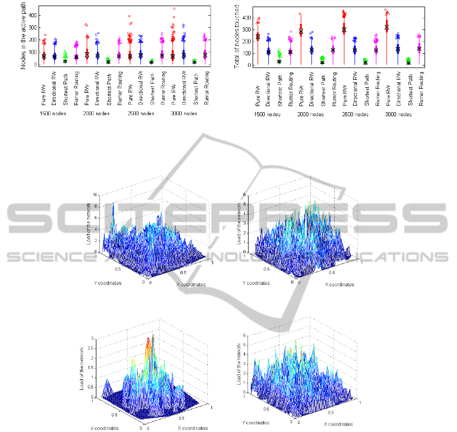
a) b)
Figure 6: Evaluation of the nodes in the active path (a) and nodes touched (b) until the intersection takes place. The following
dissemination techniques have been used: 1) PRWs, 2) DRWs, 3) Shortest Paths and 4) Rumor Routing.
a) b)
c) d)
Figure 7: Evaluation of the load of the network using the following dissemination techniques: a) PRWs, b) DRWs, c) Shortest
Paths and d) Rumor Routing.
4.2.1 Evaluation of the Intersections
In order to assure intersections, once a branch of a
DRW is stopped, we go back to the list of relaying
nodes searching for a neighbor node which is not yet
in the DRW using algorithm 3. Moreover, we have
included a mechanism that causes intersection in case
that a node detects that one of its neighbors is part of
the relaying list of nodes.
Figure 6 shows the main results obtained in this
section. The behaviour of DRWs and Rumor Rou-
ting is quite similar mainly because in Rumor Routing
we have used an infinite memory. It is remarkable to
mention that the algorithm that uses the Shortest Path
between producers and consumers is the one that uses
a smaller number of nodes. Finally, we can confirm
that PRWs use more nodes until finding an intersec-
tion.
4.2.2 Evaluation of the Load of the Network
Figure 7 shows the load of an independent and well-
connected network of 3000 nodes; 50 pairs of nodes
have been intersected. We can observe that the
method that balances better the load is the one that
uses PRWs (a). This figure shows a peak due to the

boundary effect of embedding the network. The worst
results in terms of load are obtained when using the
method of the Shortest Paths (c). We can observe that
almost all of the charge is concentrated near the center
of the network. Traditional Rumor Routing (d) with
an infinite memory and DRWs (b) present a similar
distribution of the load. It is quite balanced because
all of the nodes share the charge although some of
them are more used for dissemination than others.
5 CONCLUSION
In this paper, we have identified some of the funda-
mental issues associated to the design of an infor-
mation brokerage system for a sensor network. A
method for the solution of this problem using DRWs
has been presented.
The main result shown in this paper is that the
use of the second neighborhood in the construction
of the DRW is not efficient. It also has been shown
that the use of two branches for the construction of
the DRW improves latency achieving similar results
for depth than DRWs of one branch. Moreover, it has
been proved that higher densities of nodes in the net-
work leads to the construction of paths that use less
nodes in the list of relaying nodes. This means that
less nodes will be needed to transmit to farther zones
in the network.
In this research, we also have conducted experi-
ments to assess the suitability of our method for an
information brokerage system. The results show that
our method is good at balancing the load without
using a large amount of nodes. We prove that our
approach is similar to the use of Rumor Routing with
an infinite memory.
We can conclude that our method is suitable for
its use in an information brokerage system and that
simple strategies in the design of DRWs are efficient.
ACKNOWLEDGEMENT
This work has been developed as part of the POP-
WiN project (Parallel Object Remote Programming
for Heterogeneous Wireless Networks over IPv6) that
is financially supported by the Hasler Foundation in
its SmartWorld - Information and Communication
Technology for a Better World 2020 program.
REFERENCES
Banka, T., Tandon, G., and Jayasumana, A. P. (2005). Zonal
Rumor Routing for Wireless Sensor Networks. In
ITCC ’05: Proceedings of the International Confer-
ence on Information Technology: Coding and Com-
puting (ITCC’05) - Volume II, pages 562–567, Wash-
ington, DC, USA. IEEE Computer Society.
Braginsky, D. and Estrin, D. (2002). Rumor routing al-
gorthim for sensor networks. In Proceedings of the
1st ACM international workshop on Wireless sensor
networks and applications, WSNA ’02, pages 22–31,
New York, NY, USA. ACM.
Fang, Q., Gao, J., and Guibas, L. J. (2006). Landmark-
based information storage and retrieval in sensor net-
works. In In The 25th Conference of the IEEE Com-
munication Society (INFOCOM06, pages 1–12.
Fang, Q., Gao, J., Guibas, L. J., Silva, V., and Zhang, L.
(2005). Glider: Gradient landmark-based distributed
routing for sensor networks. In in Proc. of the 24th
Conference of the IEEE Communication Society (IN-
FOCOM, pages 339–350.
Funke, S., Guibas, L. J., Nguyen, A., and Wang, Y. (2006).
Distance-sensitive information brokerage in sensor
networks. In Proceedings of the Second IEEE interna-
tional conference on Distributed Computing in Sensor
Systems, DCOSS’06, pages 234–251, Berlin, Heidel-
berg. Springer-Verlag.
Funke, S. and Rauf, I. (2007). Information brokerage via
location-free double rulings. In Proceedings of the
6th international conference on Ad-hoc, mobile and
wireless networks, ADHOC-NOW’07, pages 87–100,
Berlin, Heidelberg. Springer-Verlag.
Leone, P. and Mu
˜
noz, C. (2013). Content based routing with
directional random walk for failure tolerance and de-
tection in cooperative large scale wireless networks.
In Proc. 2nd Intl. Workshop on Architecting Safety
in Collaborative Mobile Systems, SAFECOMP’13,
pages 313–324, Berlin, Heidelberg. Springer-Verlag.
Lin, C.-H., Kuo, J.-J., Liu, B.-H., and Tsai, M.-J.
(2012). Gps-free, boundary-recognition-free, and
reliable double-ruling-based information brokerage
scheme in wireless sensor networks. IEEE Transac-
tions on Computers, 61(6):885–898.
Liu, X., Huang, Q., and Zhang, Y. (2004). Combs, nee-
dles, haystacks: balancing push and pull for discov-
ery in large-scale sensor networks. In Proceedings of
the 2nd international conference on Embedded net-
worked sensor systems, SenSys ’04, pages 122–133,
New York, NY, USA. ACM.
Sarkar, R., Zhu, X., and Gao, J. (2009). Double rulings for
information brokerage in sensor networks. IEEE/ACM
Trans. Netw., 17(6):1902–1915.
Shokrzadeh, H., Haghighat, A. T., and Nayebi, A.
(2009). New routing framework base on rumor rou-
ting in wireless sensor networks. Comput. Commun.,
32(1):86–93.