SCLD-ATP: Symmetric Coherent Link Degree, Adaptive Transmission
Power Control for Wireless Sensor Networks
Konstantinos Chantzis
1
, Dimitrios Amaxilatis
2
, Ioannis Chatzigiannakis
2
and Jose Rolim
1
1
Centre Universitaire Informatique, University of Geneva, Genve, Switzerland
2
Computer Technology Institute and Press, University of Patras, Patras, Greece
Keywords:
Topology Control, Adaptive Protocol, Link Symmetry, Experimental Evaluation, Reliability, Fault Tolerance.
Abstract:
Wireless Sensor Networks (WSNs) are by nature dynamic and communication between sensors nodes is ad hoc.
Numerous protocols and applications proposed operate on the assumption that communication channels are
stable. Topology Control Protocols are crucial in the operation of WSNs as they adjust transmission power in
order to maintain link quality, minimize interference and provide spatial topological control. Analysis of such
protocols is performed using theoretical models that are based on unrealistic assumptions like ideal wireless
channels and perfect energy consumption and distance estimations. With these assumptions taken for granted,
theoretical models claim various performance milestones that cannot be achieved in realistic conditions. We
here present a topology control protocol that is deployable in real WSNs and distance ourselves from spatial,
temporal, environmental assumptions regarding the performance of communications on the wireless medium.
Our protocol focuses on fault tolerance and symmetric link coherence using an adaptive transmission power
scheme. From various testbed experiments we showcase the performance of SCLD-ATP in terms of load
balancing, reliability, multi-hop capabilities and power consumption.
1 INTRODUCTION
Wireless Sensor Networks (WSNs) are wireless
multi-hop networks comprised of low powered tiny
devices with limited processing capabilities and a
plethora of sensing attributes (Akyildiz et al., Aug).
This emerging and scalable technology has a vast
space of different applications like commercial and
home building automation, target tracking and health
monitoring.
In order to organize these devices into networks
that provide adequate quality of service, protocol
designers have to deal with two main problems.
First comes the problem of maintaining stable
and reliable communication between nodes. The
reliability and stability of communication in the
wireless medium is subject to many factors and
temporal qualities. These include external noise,
interference from within the network and even
hardware misconfigurations and constraints. Due to
these problems, communication quality cannot be
modeled accurately for all applications (Srinivasan
et al., 2010), (Zhao and Govindan, 2003), (Woehrle
et al., 2012). We also notice that assisting metrics
like LQI and RSSI, cannot describe accurately link
qualities in real deployments. Controlled experiments
show that equal transmission power settings from
multiple senders to one receiver and vice versa, can
also produce different link qualities between WSN
nodes (Son et al., 2004). Extensive studies show
inherent link asymmetry in WSN communications
under various settings and hardware configurations
(Misra et al., 2012). Secondly, topology control
protocols have to create and maintain sufficiently
connected, load balanced or even custom attributed
neighborhoods of nodes. Spatial control is essential
for preserving the multi-hop nature of WSNs and
minimizing radio interference and power consumption.
Solving these problems is especially hard when WSN
system installations are subjected to unpredictable
dynamicity like sudden node failures while running
applications have to sustain seamless services.
Furthermore, WSN node deployments may
be non-uniform, arbitrary, or even mobile with
the network topology varying over time. The
consequences in these cases are: a) areas where WSN
node placement is dense or sparse and communication
is redundant or with limited coverage. b) difficulty in
determining the network parameters for connectivity,
coverage and minimum energy consumption.
5
Chantzis K., Amaxilatis D., Chatzigiannakis I. and Rolim J..
SCLD-ATP: Symmetric Coherent Link Degree, Adaptive Transmission Power Control for Wireless Sensor Networks.
DOI: 10.5220/0004696200050016
In Proceedings of the 3rd International Conference on Sensor Networks (SENSORNETS-2014), pages 5-16
ISBN: 978-989-758-001-7
Copyright
c
 2014 SCITEPRESS (Science and Technology Publications, Lda.)

We focused our study towards topology control
schemes for WSNs that adjust node transmission
powers dynamically. We propose SCLD-ATP
(Symmetric Coherent Link Degree, Adaptive
Transmission Power), a protocol designed from
a perspective of providing a continuous service
that monitors and delivers sufficient, reliable
communication between WSN nodes efficiently. The
key characteristics of our proposed protocol are:
a) simplicity in terms of communication without
any deliberate organization of nodes, b) enforced
symmetry in terms of communication links for
multihop routing scenarios, c) efficient control
over connectivity and interference by adjusting the
transmission power on node level, d) fully distributed
operation, e) and lastly an abstraction over the real
network to be used by higher layer protocols or
applications.
The rest of the paper follows: In Section 2 we
present the relevant state of the art. In Section 3
we describe the general motivations of our holistic
approach while Section 4 covers the design details
of SCLD-ATP. We continue in Section 6 with
experiments and focus on link quality, load balancing,
symmetry and fault tolerance, using indoor WSN
testbeds. Last, in Section 7 we discuss future work,
possible optimizations and application schemes.
2 RELATED WORK
Topology control protocols (Santi, 2005) use
various properties of WSN nodes like transmission
power and packet rate or employ schemes like
duty cycling. Their goals range from network
construction or maintainance with various atributes
that relate to network coverage, node connectivity,
link symmetry for reliable multihop communications,
energy efficiency and interference minimization for
specicic application scenaria and traffic load. Other
schemes aim at the construction of higher level
network structures like spanning trees or hierarchical
clusters that inheritently achieve a subset of the above
atributes (Chazelle et al., 2001; Heinzelman et al.,
2000; Wang and Medidi, 2007; Blough et al., 2003;
Park and Sivakumar, 2002).
We here summarize and discuss the most
representative work related to this topic. Although our
main interest lies within real experimental research and
systems protocol design we also look at the problem of
topology control from theoretical contributions where
many ideas in recent studies of this field derived from.
Despite the fact that related work in this field uses
similar techniques and overlaps in ideas, we try to
roughly divide it in two main categories. Protocols
that prioritize on some degree of spatial conformity or
individual link quality.
2.1 Degree Based
LINT (Ramanathan and Rosales-Hain, 2000) is
a milestone attempt of distributed control, where
nodes adjust their transmission powers to maintain
a sufficient degree of neighboring nodes within a
[D
min
,D
max
] limit. The power setting for each node
is calculated as the difference between the current
power setting, to a target power setting that meets the
neighbor degree demands. This is performed using
a path-loss, receiver sensitivity and density model.
LMA and LMN (Kubisch et al., 2003) are distributed
schemes of periodic transmission power control. LMA
is based on a degree of neighbor connectedness and
LMN is based on a single degree of average neighbor
connectedness. For both of these schemes transmission
power is adjusted by a constant factor per neighbor and
link symmetry is decided based on acknowledgements.
The authors also comment on important problems of
convergence, like exclusion of nodes from stabilized
portions of the topology. DTPC (Jeong et al., 2007)
performs transmission power adjustments and link
qualification using a single RSSI threshold and a single
degree threshold. Performance of DTPC is evaluated
with experiments that focus on throughput and power
consumption.
2.2 Individual Link Based
Standalone protocols like ATPC (Lin et al., 2006) and
PCBL (Son et al., 2004) focus on fixating transmission
powers for individual links. PCBL uses a sampling
period where Packet Reception Rates (PRR) are
correlated with specific transmission power settings
for each link. Two PRR thresholds are used for
blacklisting low quality links. ATPC uses RSSI/LQI
metrics for direct link qualification. Initially RSSI
or LQI are sampled with broadcast messages and
verified for symmetry with acknowledgements. Then
a feedback loop adjusts transmission powers for
individual links, based on a least square approximation
predictive model. Alternatively ART protocol
(Hackmann et al., 2008) was designed as a lightweight
embeddedment, where topology and neighbors are
presupposed from higher level protocols. ART
computes link PRR by monitoring packets exchanged
from other protocols. Link filtering is based on
two sliding window thresholds for failure detection
correlated by two PRR values, in order to set proper
transmission power.
SENSORNETS2014-InternationalConferenceonSensorNetworks
6

3 MOTIVATION
3.1 Importance of Degree Limitations
Related work that prioritizes individual link quality
has no internal mechanism for enforcing any spatial
control over neighborhoods. We exclude ART from
this critique since it was designed as lightweight
embeddedment, where topology and neighbors are
presupposed from higher protocol layers. As far
as ATPC and PCBL are concerned, there are no
limitations to the number of links created. In a dense
node deployment these protocols will create redundant
links between nodes, maintain local maximums in
terms of neighbor connectivity and possibly subject
a high number of nodes to interference. In our
proposed protocol we follow a degree adherence of
[Dmin,Dmax] as has been provided in LINT and
LMA/LMN. Although we see that DTPC uses only
a Dmin , we believe that a Dmax is required for the
creation of load balanced neighborhoods and could
be also considered as a way of indirectly limiting
interference. A constant (Hajek, 1983), (Kleinrock
and Silvester, 1978), or dynamic (Xue and Kumar,
2004) number of neighbors (three, six or Θ(logn) )
have been proposed in order to achieve a connected
network with high probability. In our case, defining
exact degree bounds was not in our scope of interest.
3.2 Link Quality
We performed a small set of experiments in our
local testbed (UniGe) in the University of Geneva
to verify the behavior of LQI and RSSI, compared
to PRR. The testbed is currently comprised of 25
Coalesenses iSense nodes based on the 32bit Jennic
JN5139 IEEE802.15.4 wireless micro-controller that
supports six transmission power settings covering a
[−30,0] dB space, with a −6 dB step interval. We
conducted six experiments for every transmission
power setting. In all experiments nodes booted with a
random back-off timer between [0,1000] milliseconds,
to avoid collisions and broadcasted 1 beacon per
second, for 300 seconds. We observe (Fig. 1) that
when LQI and RSSI values are sampled from a
deployed network, they cannot be correlated to exact
PRR values as a general rule. Also, high PRR links
can exist inside the full LQI and RSSI value spectrum.
Different obstacles, equipment that generate noise and
temporal environmental conditions between individual
links, can alter the RSSI or LQI of a considerable
amount of links that hold high PRR values. In Fig. 2
we also see that link length does not correlate with
specific LQI and cannot produce a clear approximation
0
0.2
0.4
0.6
0.8
1
0 50 100 150 200 250
PRR
Average RSSI
0dB
-6dB
-12dB
-18dB
-24dB
-30dB
0
0.2
0.4
0.6
0.8
1
0 50 100 150 200 250
PRR
Average LQI
0dB
-6dB
-12dB
-18dB
-24dB
-30dB
Figure 1: Link PRR versus average LQI and RSSI. Each
point represents a link in a transmission power.
0
20
40
60
80
100
120
140
160
0 5 10 15 20 25
Average RSSI
Distance
0dB
-6dB
-12dB
-18dB
-24dB
-30dB
0
50
100
150
200
250
0 5 10 15 20 25
Average LQI
Distance
0dB
-6dB
-12dB
-18dB
-24dB
-30dB
Figure 2: Average LQI and RSSI versus link length. Each
point represents a link in a transmission power setting.
for RSSI values for the first 10 meters. Strategies
that include certain value ranges as “close distance”
links, or exclude values as “long distance” links would
not be accurate. We do agree that RSSI and LQI
could be correlated with specific PRR values, but only
on an individual link basis and only under specific
environmental conditions.
3.3 Fault Tolerance
An important aspect of topology control protocols,
is the detection of abrupt changes in the topology,
before they could potentially hinder the performance
of higher layer protocols. For example, an unhandled
node failure at an arbitrary moment in time would
cause a failure for a routing scheme and maximum
retransmissions, if the faulty node was chosen as the
next recipient. Topology control schemes that utilize
PRR as a link quality descriptor will have to update the
failure through PRR convergence. If PRR is derived
through a high number of accumulated messages, PRR
updates per message would take a considerable amount
of time in order to reflect the failure (like PCBL). In the
case of ART the failure will be detected via the double
sliding window of failures, but due to the embedded
nature of ART, the detection will come after failure.
SCLD-ATP:SymmetricCoherentLinkDegree,AdaptiveTransmissionPowerControlforWirelessSensorNetworks
7

4 SCLD-ATP DESIGN
4.1 Link Quantification
We focus on PRR for link characterization, but this
information does not guarantee equal behaviour on
a bidirectional basis. Protocols like PCBL and
ART correlate the ability for successful delivery of
a message from node A to node B, to the ability of
node A receiving a message from node B. ART verifies
this with acknowledgements after a successful unicast
reception from node A to node B. SCLD-ATP on the
other hand provides nodes with their inverse PRR
( inv PRR ). A link between node A and node B is
characterized by two PRR values, PRR
A
calculated
locally in node B and PRR
B
calculated locally in
node A. In fact PRR
A
calculated in node B is more
important for node A than PRR
B
, as it represents the
exact capability of node A delivering a message to
node B. PRR
A
for node A is the inv PRR
B
of the link.
Figure 3: The online service scheme of SCLD-ATP.
4.2 Online Service
In SCLD, we follow a stand alone protocol scheme
that acts as an online service (Fig. 3). Initially
nodes broadcast beacon messages at a constant but
also locally adjustable rate. Specifically a packet is
broadcasted with a uniform random back-off timer
once in every broadcast period. When nodes receive
beacons from their neighbors, they store their unique
ID’s, update their PRR and also maintain averages for
LQI and RSSI. Since the beacon rate is advertised in
the broadcasts, recipients can dynamically calculate
the number of expected messages that affect PRR
and average RSSI and LQI. Based on user or
higher protocol parameters, links with high PRR are
advertised in the beacons. Specifically, nodes include
the ID’s as well as the updated PRR of their neighbors
in their messages. Receivers that find themselves in
broadcast messages, acquire these inv PRR values
and update the link information between them and
the sender locally. After a predefined number of
beacons that produce a stable PRR, a monitoring
phase, the SCLD-ATP daemon kicks in and assesses
quality and number of links. All links must exceed two
PRR thresholds {T h
PRR
,T h
inv PRR
} to be considered
symmetric. Nodes must also contain a bounded degree
of these links between [D
min
,D
max
] . If the degree of
these links is lower than D
min
, the transmission power
of the node is increased by one step. If the degree
of these links is higher than D
max
, the transmission
power is decreased by one step. We see this in the
Transmission power adjustment instances in Fig. 3.
After the transmission power adjustment, a new PRR is
computed for all links based on an exponential moving
average with a high coefficient. This also applies for
LQI and RSSI averages.
A
B
Trans. Power Reduction
B 90% 90%
Neigh.ID PRR inv.PRR
Trust inv.Trust
Neighbor List of Node A
B 90% 90%
staleslow conv.
B 90% 90%
staleslow conv.
Node A Bcast
Neigh.ID inv.PRR
B 90%
Node B Bcast
Neigh.ID inv.PRR
A 90%
A 90% 90%
Neigh.ID PRR inv.PRR
Trust inv.Trust
Neighbor List of Node B
A 90% 90%
false
A 90% 90%
false
Node A Bcast
Neigh.ID inv.PRR
B not included
Node B Bcast
Neigh.ID inv.PRR
A 90%
B
T
<T
TH
B
T
<T
TH
T
B
<T
TH
inv.
T
B
<T
TH
inv.
T
A
<T
TH
inv.
T
A
<T
TH
inv.
T
MAX
T
MAX
T
MAX
T
MAX
T
MAX
T
MAX
Figure 4: Loss of symmetry is detected in both sides.
Neighbor B is not considered for Node A due to T
B
≤ T
T H
and not included in broadcasts. Neighbor A is not considered
for Node B due to inv T
A
≤ T
T H
, but included in broadcasts
as fit.
4.3 Symmetric Coherent Links
Nodes in SCLD-ATP simply broadcast
information autonomously, without depending
on acknowledgements from other nodes. Changes
that could affect the quality of symmetry in links
could happen during abrupt dynamics and failures,
or increases and decreases of transmission power
during normal operation. PRR and inv PRR are
not sufficient enough to characterize a link in this
case. In fact, a message reception or it’s expectancy
can always contribute towards the computation of
a statistic like PRR. On the other hand, statistics
regarding conditional information (like inv PRR)
within a message cannot be computed in the same
way. Since inv PRR has to be computed by a neighbor
and cannot always be delivered, its value has to be
characterized as trustworthy by the recipient. We will
describe this necessity from the example of Fig. 4.
SENSORNETS2014-InternationalConferenceonSensorNetworks
8

We see that node A maintains information about
node B {PRR
B
,inv PRR
B
} and node B maintains
information about node A {PRR
A
,inv PRR
A
} . The
symmetric link is stable at {90%,90%} from both
perspectives. At an arbitrary moment, node B decides
to reduce it’s transmission power enough to sever
the symmetry of the link. Node A can deliver
messages normally to node B, but node B cannot
deliver messages to node A and thus cannot send
PRR
A
to node A. In the mean time PRR
B
will start to
slowly converge towards the actual behaviour of node
B. inv PRR
B
on the other hand cannot be updated by
node A and will remain stale. Without any control of
this situation, node A would still advertise symmetry
to node B, until PRR
B
finally gets under a minimum
threshold. Since node B is always able to receive
messages from node A, it will still assume symmetry
in the link and will continue to maintain node A as a
viable neighbor. We propose a simple and effective
solution to this problem in the form of a trust based
mechanism:
(a) A trust value T to regulate PRR with
T ∈ [T
min
,T
max
] . T accumulates per successful
message, reduces per failed delivery.
(b) A trust value inv T to regulate inv PRR with
T ∈ [T
min
,T
max
] . inv T accumulates per successful
delivery of inv PRR information , reduces on non
delivery.
(c) A threshold T
T H
=
T
min
+T
max
2
(d) A link is symmetric and coherent ( SCL ) when
both T > T
T H
and inv T > T
T H
.
Following this scheme we see that as soon as node
B can’t deliver messages, T
B
falls below the T
T H
threshold and the link is not considered as viable, nor it
is included in the broadcast messages of node A. Node
B on the other hand maintains high T
A
for node A, but
since there is no delivery for inv PRR
A
the link is not
considered viable as well. Still, since the link is trusted
to deliver information (or the knowledge of lack of
information), node A is included in the broadcasts of
node B. We will be referring to the degree of SCLs in
a node as SCLD, the nodes that contain an SCLD less
than the D min threshold as local SCLD minimums,
while the nodes that contain an SCLD higher than the
D max threshold as local SCLD maximums.
4.4 Spatial Control
An important choice we followed with SCLD-ATP,
is to include upper and lower bounds [D
min
,D
max
] for
the links delivered (like LINT and LMA/LMN) and
not a single D
min
threshold (like DTPC). The reason
lies within the fact that it is very hard for nodes to
converge to an equal, exact degree threshold. In the
case of our iSense nodes, the difference between two
settings of transmission power is so large that a single
degree threshold could cause oscillating behaviour
between two transmission power settings. The low
setting would never be able to achieve a degree higher
than D
min
and the high setting will always achieve a
degree higher than D
min
. Later in our experiments we
will see that when degrees are unattainable, oscillating
behaviour could potentially spread to all the nodes in
a topology.
Unlike DTPC but similarly to TPSO, we choose
to start the convergence process with the minimum
transmission power setting for all nodes. In
deployments where nodes boot with the maximum
transmission power setting, links of various lengths
are going to antagonize for a position in the limited
[D
min
,D
max
] space that their neighbors have to
maintain. Since the criteria of reducing transmission
power is related to the degree of high quality links,
a high setting that could fullfil degree requirements
for some nodes, could be unecessary. The same
requirements could be achievable with some lower
setting. Also starting with the lowest setting means
that link qualification in monitoring phases will start
with minimum interference.
An important feature of SCLD-ATP is the
ability to mitigate the effects of node exclusion in
converged neighborhoods. As previously discussed,
a [D
min
, D
max
] limit enforces antagonism on links.
Since we start with the minimum transmission power
on all nodes, we always favor the shortest available
links. This introduces problems in terms of the general
connectedness of the topology and more specifically
introduces node exclusion. For example, a network
could contain disconnected nodes. Normally these
nodes will start increasing their transmission power
in order for their beacons to be discovered by other
nodes. If all the recipients have converged to their
SCLDs with a relatively low transmission power
setting, they will show no interest in increasing their
transmission power any further. Thus, excluded nodes
could continue being excluded from participating in
symmetric and coherent links. To mitigate this effect,
all nodes advertise their SCLD in their beacons. A
receiving node stores this information for all links
and before each beacon, the links maintained by a
node are sorted by their advertised SCLD. Priority
is given to the first D
min
number of links with the
least SCL Degree . Transmission power could then be
increased further, to serve the “most desperate” nodes
first. With this technique, the priority of maintaining
shortest links can be overridden by the presence of
excluded or less connected nodes.
SCLD-ATP:SymmetricCoherentLinkDegree,AdaptiveTransmissionPowerControlforWirelessSensorNetworks
9

0
5
10
15
20
0 5 10 15 20
number of nodes
monitoring phase
local SCLD minimums
local SCLD maximums
Figure 5: Oscillating SCLD local minimums and maximums.
Stabilization is impossible when a narrow [2, 3] SCLD range
is chosen.
-35
-30
-25
-20
-15
-10
-5
0
5
0 2 4 6 8 10 12 14 16 18
transmission power (dB)
monitoring phase
-1
-0.5
0
0.5
1
0 2 4 6 8 10 12 14 16 18
ACF
k-lag
Figure 6: Oscillation detection on a single node. From
feedback setting as a discrete time series, to normalized
correlogram and in the end, peak detection.
4.5 Feedback Oscillations
This problem of oscillations in transmission power was
initially observed after the duration of experiments
by sampling the networks number of local SCLD
minimums and maximums for each monitoring phase.
As seen in Fig. 5, oscillations could potentially affect
the complete topology. In order to mitigate their
effects, we first had to detect them at a node level.
We use a rolling history window for both
transmission power adjustments and correlated SCLD
values and treat them as discrete time series with
samples taken every monitoring phase. When the
history window of transmission power adjustments
is full (ten samples in our case), we perform an
autocorrelation. This local computation takes place
on every monitoring phase and is normalized by
mean and variance for a five sample frame. In this
way a temporary correlogram can be produced on
memory. By detecting peaks inside this correlogram,
we can expose cases of hidden periodicity. Any
autocorrelation coefficient higher than two times
the variance of the history window, is considered
a peak. Fig. 6 shows the transmission power
adjustments of a single node in the topology when
an oscillating behaviour occurs. When three or
more peaks are detected, we simply increment
D max and decrement D min . Nevertheless, not all
oscillations are problematic. During convergence,
nodes might oscillate between high and low
settings until they stabilize, as seen in the local
SCLD minimums/maximums graph from Fig. 18.
SCLD-ATP only regulates the oscillations that show
a non stabilizing behaviour, signified by peaks in the
corellogram that either have monotonous increasing
or constant absolute values.
5 IMPLEMENTATION
We implement our protocol using Wiselib
(Baumgartner et al., 2010): a code library, that
allows implementations to be OS-independent.
It is implemented based on C++ and templates,
but without virtual inheritance and exceptions.
Algorithm implementations can be recompiled for
several platforms and firmwares, without the need to
change the code. Wiselib can interface with systems
implemented using C (Contiki), C++ (iSense), and
nesC (TinyOS). Additionally, Wiselib also runs
on the simulator Shawn (Fekete et al., 2007) and
TOSSIM (Levis et al., 2003), hereby easing the
transition from simulation to actual devices.
SCLD-ATP is designed (Fig. 7) as two
closely-coupled software modules. The first module,
named SCL , is responsible for: a) performing the
periodic broadcasts, b) maintaining and updating
neighborhood lists, c) filtering links based on
thresholds, d) providing an API for dynamic threshold
updates. The second module, named ATP acts as a
daemon that periodically accesses and assesses the
neighborhood list of SCL module. Based on the
quality and quantity of links, the transmission power
is increased, decreased or remains constant.
Our implementation is also based on the Unifying
Link Abstraction Layer (Polastre et al., ) principle
and Wiselib’s Topology Control Concept. We thus
provide an abstract interface for interaction and
asynchronous communication with the established
topology that other developers can use to implement
their own protocols without hassle. In more detail,
SCLD-ATP acts as intermediate service between the
actual hardware radio communication and higher layer
protocols and applications. Using Wiselib’s generic
callback mechanisms other protocols can register and
receive notifications and information whenever the
topology is altered.
Additionally we offer a reliable broadcasting
mechanism for message exchanges over the
established neighborhoods. This mechanism takes
advantage of SCLD-ATP’s periodic beaconing process
and piggybacks external payloads on its messages.
SENSORNETS2014-InternationalConferenceonSensorNetworks
10

As a result other applications including clustering,
grouping or tracking can be implemented with less
dedicated message exchanges, reducing both the
network traffic and energy consumption.
RADIO
SCLD-ATP PROTOCOL
SCL module
ATP module
Neighborhood List
Transmission
Power Setting
Registration
Callbacks
Registered
Protocol
Threshold
Settings
List
Periodic Transmission
Power adjustment
Link
Assessment
Link Information
Packets
Link
Information
Requests
Routing
Dissemination
Target Tracking
Localization
…..
…..
Figure 7: SCLD-ATP modular and interactive design. High
layer protocols can register for callbacks to receive updates
and also access link information on demand.
5.1 State of the Art Implementation
We have also implemented the degree based protocols
discussed in Section 2.1, namely DTPC (Jeong et al.,
2007), LINT (Ramanathan and Rosales-Hain, 2000)
and LMA/LMN (Kubisch et al., 2003). As far as
DTPC is concerned, implementation was simply a
choice of parameters and optimizations being disabled.
Since LMA/LMN were theoretical protocols, we
deviated from their design in favor of implementation.
Instead of using the two distinct packet types for
symmetry (for every broadcast message all receivers
must send acknowledgement packets), we used our
single beacon packet scheme and included the LMN
heuristics for average neighbor connectedness.
LINT, also a theoretical scheme, was designed
for instant and not incremental transmission power
adjustments based on a path-loss model. We
first implemented a log-normal shadowing model
(Stojmenovic et al., 2005), for fast computations of
the probability of reception PR
S
and parameterized it
to match the capabilities of our iSense nodes, with
six different transmission power settings. For the
distance to transmission power correlation we used
a simplification of the Friss free range propagation
model (Rappaport, 1996) where R = 50 · 10
P
T X
20
. We
have also added a uniform random irregularity factor
r
f
∈ [0,0.15] such that PR = PR
S
(1 − r
f
) , as seen in
Fig. 8. The beacon packet was also updated so that
nodes include their transmission power setting in dB.
A node running the LINT protocol starts increasing
its transmission power until it acquires a number
of neighbors bounded by [D min,D max] . Then, it
performs a quick-sort on its neighbor list based on
PRR. If the PRR of the (D min)th neighbor is below
0
0.2
0.4
0.6
0.8
1
0 10 20 30 40 50
Probability of Reception
Distance (m)
-30dB
-24dB
-18dB
-12dB
-6dB
0dB
Figure 8: Log-normal shadowing model for LINT
implementation.
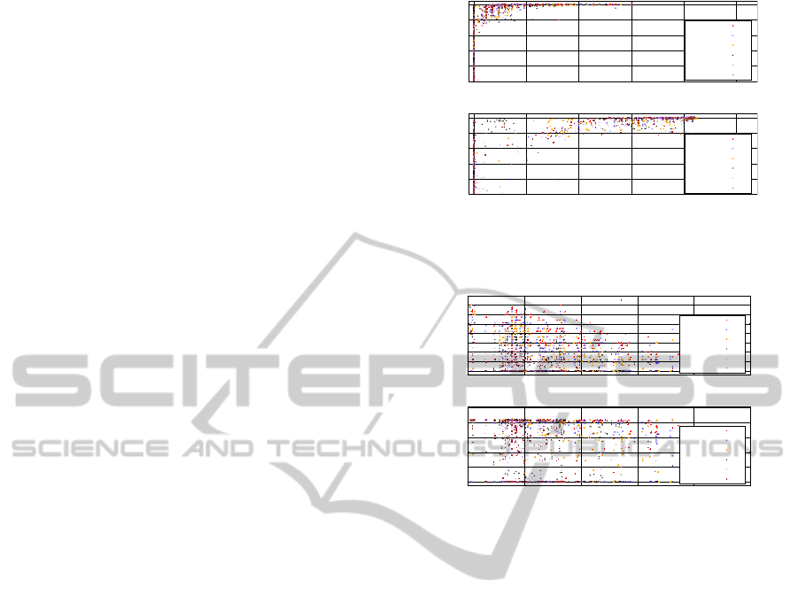
Table 1: The broadcast packet of SCLD-ATP.
Data size in bytes
Message ID 2
Node ID 2
Beacon Rate (ms) 2
Symmetric Coherent Link Degree 1
Length of neighborhood list (bytes) 1
Length of custom payload list (bytes) 1
Neighborhood list
Node ID 2
inv PRR 1
average inv LQI 1
average inv RSSI 1
. . . . . . . . . . . . . . . . . . . . . . . .
Custom payload list
length of custom payload (bytes) 1
custom payload variable
. . . . . . . . . . . . . . . . . . . . . . . .
a certain PRR threshold, it approximates its distance
using its advertised transmission power setting from
the radio propagation model. Then, it finds the lowest
transmission power setting for packet delivery above
the PRR threshold, at that given distance. Since
transmission power is increased to meet the demands
for the node with the lowest PRR (and thus the more
distant), it will also cover the demands of the first
(D min − i)th neighbors.
5.2 Constrained by Resources
The size of the final binary file we flashed in our
iSense nodes was approximately 60KB for all cases.
With 40KB for the standard firmware including the
WISELIB interface instances (such as Radio, Debug,
Rand, Clock, Timer), 14KB for the SCL module
and approximately 4KB for the ATP module. Each
entry in the neighborhood list maintained in the SCL
module is 24 bytes, while a single entry for the
registered protocol buffer occupies 17 bytes without
any additional custom payload data. For a topology
of 25 neighbors and 1 registered protocol we had to
allocate less than 1KB of memory.
SCLD-ATP:SymmetricCoherentLinkDegree,AdaptiveTransmissionPowerControlforWirelessSensorNetworks
11

As far as the packet size is concerned (Table 1),
based on the maximum size of 116 bytes we use a
header of 9 bytes. Each symmetric trusted (SCL)
neighbor occupies a maximum of 5 bytes with a
maximum of 21 neighbors per packet, or 3 bytes
if we exclude average inverse MAC metrics with a
maximum of 35 neighbors per packet. If protocols
register with custom payloads, less neighbors are
going to fit inside a single packet. Threshold
limitations on link quality in conjunction with the least
SCLD optimization could further reduce the need of
occupying valuable packet space.
6 REAL EXPERIMENTS
For our real device experiments we used the testbeds
of the WISEBED flexible experimentation framework
(Coulson et al., 2012). UniGe previously discussed
in Section 3 and CTI testbed (Computer Technology
Institute and Press University of Patras) that contains
11 iSense nodes. We assess the performance of our
protocol and compare it to the state of the art in terms
of:
• Network consistency. A topology that
maintains a minimum number of local SCLD
minimums/maximums is load balanced, fault
tolerant and harder to partition.
• Average transmission power of the topology, as a
factor of power consumption and interference.
• Multi-hop performance. At the end of each
experiment we inject 10 agent-packets that perform
a random walk in the topology using a 2-max
retransmission scheme. We consider a protocol
suitable for multi-hop strategies when the average
number of agent hops is above 5000.
The experiment settings were: a [4,6] degree range,
PRR and inv PRR thresholds at 90% and trust
thresholds [T
min
,T
max
] at [0,6] . All nodes broadcast
one packet per second and boot from the minimum
transmission power setting (−30dB) , unless stated
otherwise. Each monitoring phase lasts for 20 seconds.
6.1 DTPC Performance
In order to recreate DTPC with our design, we disabled
average RSSI and average inv RSSI filtering (replaced
by the newest received values), oscillation detection,
as well as the the D max upper bound. A node adjusts
its transmission power based on a single threshold of
(D min + D max)/2.
We conducted various experimental runs for DTPC
and chose to initially report results based on two RSSI
threshold settings. The first setting considers links with
RSSI ≥ 20 and inv RSSI ≥ 20 and produces a topology
that maintains an average transmission power setting at
approximately −20dB . The second setting considers
links with RSSI ≥ 50 and inv RSSI ≥ 50 to ensure
that all links maintain a PRR and inv PRR above 90%
based on Fig. 1.
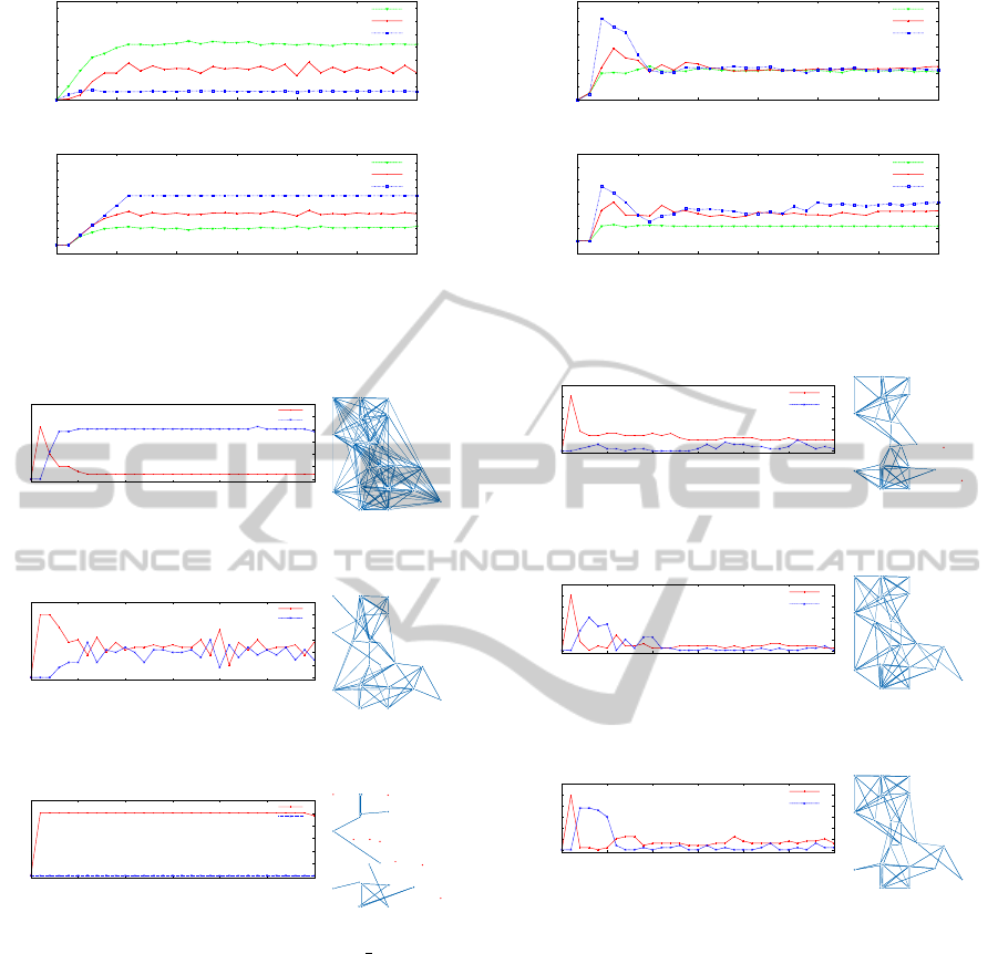
Results presented in Fig. 9 show that the DTPC-20
considers many links of questionable performance
that result in an average link degree around 8 for
the topology. Fig. 10 shows that the topology
maintains a high number of local degree maximums.
Agents injected later, couldn’t complete the first 5
hops in their traversal. DTPC-50 on the other hand
showed an average link degree close to the D min
threshold with increased transmission power around
−10dB . Still, Fig. 11 shows a continuous high
number of local degree minimums and maximums
and similar poor performance in multihop attempts.
Further investigation showed great instability and
oscillations on individual node level. Both cases are
problematic because: a) RSSI cannot correlate to a
specific PRR value accurately. Thus symmetry using
plain RSSI values doesn’t correlate to true symmetry.
b) Transmission power adjustments as well as normal
beaconing operations can cause high RSSI fluctuation.
c) A single degree threshold that is unatainable on
the lowest transmission power adjustment difference,
will cause oscillations that could extend to other
nodes (Fig. 11). For the last experiment in this
set, we enhanced DTPC to support averages for
RSSI , inv RSSI as well as symmetric trust. We kept
the average RSSI threshold at 50. Results in Fig. 12
coincide with Fig. 1. This time many links of good
PRR performance are not considered for this RSSI
threshold even with all nodes transmitting at maximum
setting (0dB) . Alternatively all agents performed well
above the 5000 hops, trapped in the lower section of
the topology.
6.2 LINT/LMA/LMN Performance
Conducting experiments with LMA/LMN produced
poor results on on all aspects resembling the case of
DTPC-20 in Fig. 10. Since we were further interested
in the heuristics of LMN, we enhanced it with the
SCL qualification criteria. Nodes running the LMN+
protocol increase or decrease their transmission power
based on the average SCLD of their neighbors, thus we
treated the SCLD threshold as the average SCLD of
neighbors threshold. Subsequent results in Fig. 13, 14
showed an extremely low average transmission power
setting for the topology, approximately one third of the
network nodes as local SCLD minimums as well as
SENSORNETS2014-InternationalConferenceonSensorNetworks
12

0
2
4
6
8
10
12
14
0 5 10 15 20 25 30
number of nodes
monitoring phase
DTPC (RSSI>20)
DTPC (RSSI>50)
DTPC+ (avg RSSI>50, trust)
-35
-30
-25
-20
-15
-10
-5
0
5
10
15
20
25
0 5 10 15 20 25 30
transmission power (dB)
monitoring phase
DTPC (RSSI>20)
DTPC (RSSI>50)
DTPC+ (avg RSSI>50, trust)
Figure 9: Average Degree for DTPC, average SCLD for
DTPC+ and average transmission power for the different
RSSI/trust settings.
0
5
10
15
20
25
30
0 5 10 15 20 25 30
number of nodes
monitoring phase
local degree minimums
local degree maximums
Figure 10: DTPC: Local degree minimums/maximums and
link graph at 30th monitoring phase, with RSSI ≥ 20.
0
5
10
15
20
25
30
0 5 10 15 20 25 30
number of nodes
monitoring phase
local degree minimums
local degree maximums
Figure 11: DTPC: Local degree minimums/maximums and
link graph at 30th monitoring phase, with RSSI ≥ 50.
0
5
10
15
20
25
30
0 5 10 15 20 25 30
number of nodes
monitoring phase
local degree minimums
local degree maximums
Figure 12: DTPC+: Local SCLD minimums/maximums and
SCL graph at 30th monitoring phase, with AV G RSSI ≥ 50
and symmetric trust.
some nodes being completely disconnected from the
topology. Nevertheless, the SCL provisions allowed
agents to traverse successfully with an average number
of hops above 5000.
For LINT, all notions of link symmetry were
disabled. Results showed very good performance
for degree convergence and low average transmission
power (approximately -20dB) for the topology. Still
all agents could not complete the necessary number
of hops. Upon enabling SCL provisions, LINT+
maintained a performance of SCLD convergence with
multihop attempts fulfilling an average 5000 hops. The
trade-off was an increase in the average transmission
power (-15.2dB) and few local SCLD maximums.
0
2
4
6
8
10
12
14
0 5 10 15 20 25 30
number of nodes
monitoring phase
LMN+
LINT
LINT+
-35
-30
-25
-20
-15
-10
-5
0
5
0 5 10 15 20 25 30
transmission power (dB)
monitoring phase
LMN+
LINT
LINT+
Figure 13: Average Degree for LINT, average SCLD for
LINT+/LMN+ and average transmission power.
0
5
10
15
20
25
30
0 5 10 15 20 25 30
number of nodes
monitoring phase
local degree mins
local degree maxs
Figure 14: LMN+: Local SCLD minimums/maximums and
SCL graph at 30th monitoring.
0
5
10
15
20
25
30
0 5 10 15 20 25 30
number of nodes
monitoring phase
local degree mins
local degree maxs
Figure 15: LINT: Local degree minimums/maximums and
link graph at 30th monitoring phase.
0
5
10
15
20
25
30
0 5 10 15 20 25 30
number of nodes
monitoring phase
local degree mins
local degree maxs
Figure 16: LINT+: Local SCLD minimums/maximums and
SCL graph at 30th monitoring phase.
6.3 SCLD-ATP Performance
We performed three runs for SCLD-ATP. On the
first run, nodes boot with the maximum transmission
power (0dB), on the second run with the minimum
transmission power (-30dB) and on the last run, nodes
boot with a random transmission power setting.
In Fig. 17 we see that all variations produce very
similar results as they converge to the same average
SCLD well inside the [D
min
,D
max
] range. Random and
minimum transmission power boot settings maintain a
low average transmission power at −20dB while the
maximum transmission power boot setting maintained
a −16.2dB average setting. Local SCLD minimums
and maximums also tend to become minimal in Fig. 18
19, 20. Multihop performance was also successful with
SCLD-ATP:SymmetricCoherentLinkDegree,AdaptiveTransmissionPowerControlforWirelessSensorNetworks
13

0
4
8
12
16
20
24
28
0 5 10 15 20 25 30
number of nodes
monitoring phase
SCLD-ATP (boot -30db)
SCLD-ATP (boot -0db)
SCLD-ATP (boot random db)
-35
-30
-25
-20
-15
-10
-5
0
5
10
15
0 5 10 15 20 25 30
transmission power (dB)
monitoring phase
SCLD-ATP (boot -30db)
SCLD-ATP (boot -0db)
SCLD-ATP (boot random db)
Figure 17: SCLD-ATP: Average SCLD and average
transmission power for different boot settings.
0
5
10
15
20
25
30
0 5 10 15 20 25 30
number of nodes
monitoring phase
local SCLD minimums
local SCLD maximums
Figure 18: SCLD-ATP: Local SCLD minimums/maximums
and SCL graph at 30th mon. phase, booting from 0dB.
0
5
10
15
20
25
30
0 5 10 15 20 25 30
number of nodes
monitoring phase
local SCLD minimums
local SCLD maximums
Figure 19: SCLD-ATP: Local SCLD minimums/maximums
and SCL graph at 30th mon. phase, booting from -30dB.
0
5
10
15
20
25
30
0 5 10 15 20 25 30
number of nodes
monitoring phase
local SCLD minimums
local SCLD maximums
Figure 20: SCLD-ATP: Local SCLD minimums/maximums
and final SCL graph, booting from a random setting.
agents performing above 5000 hops on all cases.
From comparisons we see SCLD-ATP outperforms
DTPC. At an equal average transmission power setting
of approximately −20dB , DTPC fails to maintain a
low number of local degree minimums and maximums
and performs poorly in multihop attempts. With
a higher RSSI filtering DTPC fails similarly with
additional oscillations. Even when an average RSSI
threshold guarantees links of high quality (DTPC+), it
filters out a significant amount of links that do indeed
perform well but are not correlated accurately to RSSI.
Comparing the performance of LMN+ we see that
it does operate at a lower transmission power setting
at −24dB but the heuristics used tend to make nodes
not care about their degrees and result in a significant
number of local SCLD minimums as well as nodes
being completely excluded. Running LINT without
any SCL provisions performed poorly in multihop
attempts. LINT+ showed good results on all levels as
it maintained low local SCLD minimums/maximums,
excellent multihop performance and an average
transmission power at a −15dB margin, closely related
to the innability of the path-loss model to describe
accurately properties of different links. Still, the
default setting of SCLD-ATP (boot at 0dB ) results
in an average of −20dB, a scale lower.
Since our hardware nodes didn’t support energy
monitoring, we coupled one node with a battery sensor
and an AA battery ( 2250mAh ) and programmed it with
version of SCLD-ATP to run at fixed transmission
power settings. The node was reporting battery
capacity statistics via broadcasts and was subjected to
8 packets per second. A second node that provided the
packets was receiving and logging statistics. Hourly
operations showed linear battery drain of 39750uAh
at −30dB , 40125uAh at −24dB and 40250uAh at
−18dB . A WSN topology running SCLD-ATP with
single AA batteries on iSense nodes, at an average
−20dB , without any duty cycling scheme could last
for approximately 55 hours of continuous operation.
6.4 Topology Repair and Fault
Tolerance
Here we show how a disconnected network could be
repaired and secondly, the ability of the SCLD-ATP
protocol to recover from abrupt node failures. First, we
try to create a scenario of disconnectedness through
convergence. We perform our tests using the CTI
testbed but enforce a [2,3] SCLD limit and run
the experiment for 60 monitoring phases. At the
30th monitoring phase we enable a middle-node
between these neighborhoods. As seen in Fig. 21,
the topology is divided into two disconnected
neighborhoods. Nodes in these neighborhoods have
sufficient SCLDs and have no interest whatsoever to
increase their transmission power further. Since the
newly introduced node has no SCLs, it advertises
a SCLD equal to zero in its broadcasted beacons.
As soon as the middle-node becomes trusted to its
unwilling to connect neighbors, its SCLD is treated
with higher priority due to the least SCL optimization.
At latter, phases SCLs are regulated again based
on the [D
min
,D
max
] thresholds with the excessive
SCLs destroyed. In the end, the topology stabilizes
with a low number of SCLD local minimums and
maximums and a stable average transmission power
setting (Fig. 22).
We continue with our next experiment in the UniGe
testbed. The number of monitoring phases is set to 60
and all the nodes start from the minimum transmission
SENSORNETS2014-InternationalConferenceonSensorNetworks
14

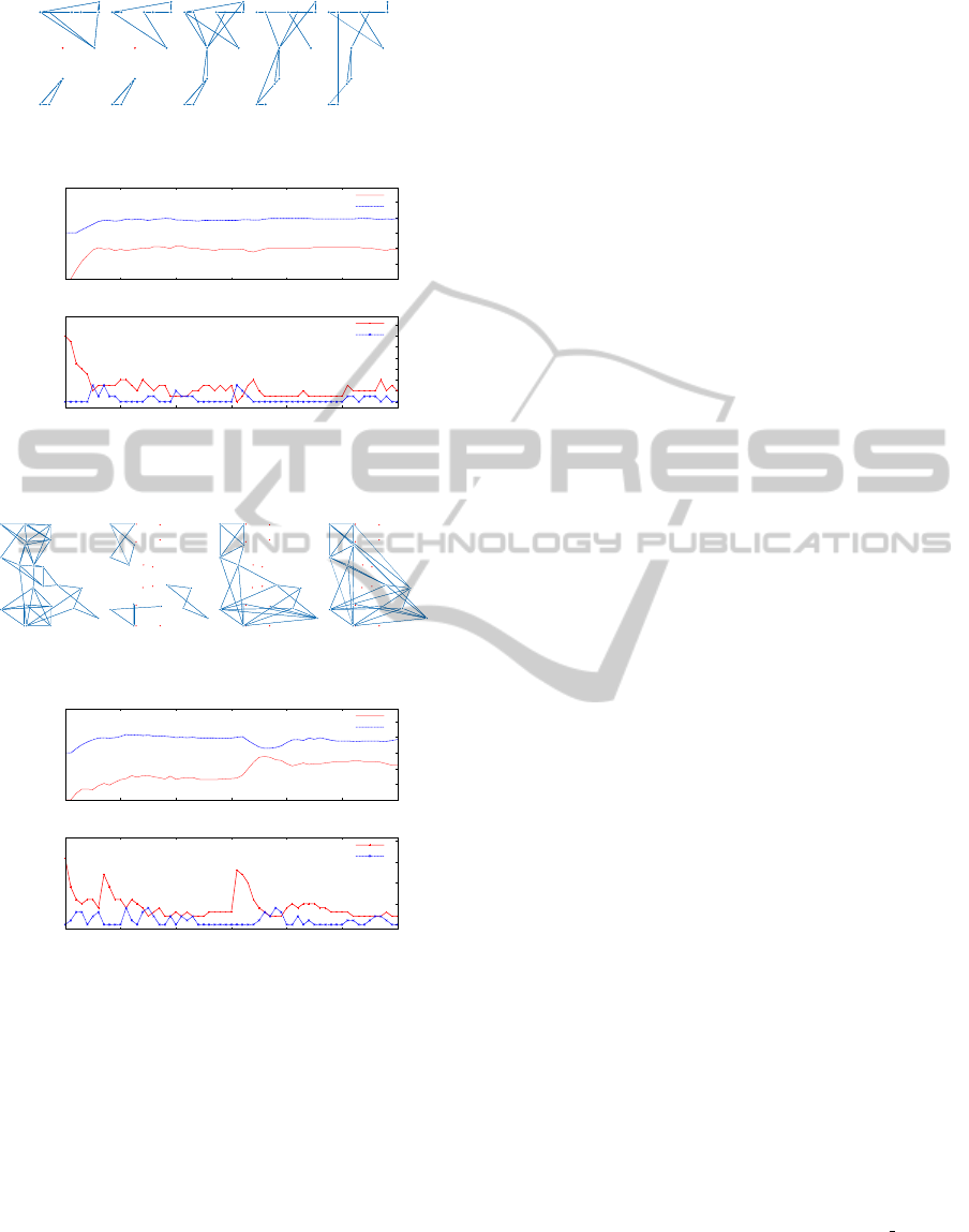
Figure 21: SCL graph transition, before and after enabling
middle-node.
-30
-20
-10
0
10
20
0 10 20 30 40 50 60
transmission dB
monitoring phase
avg dB : -11
stdev dB : 9.11043
avg dB
stdev dB
0
2
4
6
8
10
12
14
0 10 20 30 40 50 60
number of nodes
monitoring phase
local SCLD minimums
local SCLD maximums
Figure 22: Average transmission power and local SCLD
minimums/maximums booting from 0dB.
Figure 23: SCL graph transition, before and after disabling
middle section.
-30
-20
-10
0
10
20
0 10 20 30 40 50 60
transmission dB
monitoring phase
avg dB : -7.84615
stdev dB : 8.60989
avg dB
stdev dB
0
5
10
15
20
0 10 20 30 40 50 60
number of nodes
monitoring phase
local SCLD minimums
local SCLD maximums
Figure 24: Average transmission power and local SCLD
minimums/maximums booting from 0dB.
power setting with a [4,6] SCLD range. At the
30th monitoring phase we shut down 12 nodes in
the middle section. From Fig. 23 we observe that
nodes initially form an SCL connected topology until
the 30th monitoring phase. Then, the selected nodes
are disabled and the topology is divided. After three
monitoring phases, the network resumes an adequate
SCLD within the predefined range and remains stable.
Since the disabled nodes split the topology to distant
parts, new SCLs have higher lengths and correlate to
higher transmission powers, thus reflecting the average
transmission power increase (raised by 10dB). Lastly,
local SCLD minimums and maximums stabilize in low
numbers with a spike of local minimums at the 31st
monitoring phase (Fig. 24)
7 CONCLUSIONS AND FUTURE
WORK
In this paper we have presented SCLD-ATP, a topology
control protocol with adaptive transmission power
adjustments that operates as a ubiquitous service.
Its main functionality is to create, maintain and
constantly update a load balanced, stabilized network
for low transmission power operation, that maintains
multihop capabilities. It also provides a general
network abstraction, so higher layer protocols can be
updated via callbacks or on-demand requests for link
information. Through various experiments we show
that SCLD-ATP can tackle many inherent problems
of WSNs such as unreliable and asymmetric links,
network instability and unpredictable events.
We wish to extend our proposed protocol
for adaptive throughput control, perform further
experiments with mobile nodes and test it in
conjunction with other protocols like routing or
target tracking. Other ideas include heuristics for
transmission power adjustment on neighborhood
weighted local SCLD minimums and maximums
minimization.
ACKNOWLEDGEMENTS
The authors would like to thank Tigran Tonoyan for
his insightful comments. This project was supported
by the EU project HOBNET - ICT/FIRE STREP
257466.
REFERENCES
Akyildiz, I., Su, W., Sankarasubramaniam, Y., and Cayirci, E.
(Aug). A survey on sensor networks. Communications
Magazine, IEEE, 40(8):102–114.
Baumgartner, T., Chatzigiannakis, I., Fekete, S., Koninis,
C., Kr
¨
oller, A., and Pyrgelis, A. (2010). Wiselib:
A generic algorithm library for heterogeneous sensor
networks. In Wireless Sensor Networks, volume 5970
of Lecture Notes in Computer Science, pages 162–177.
Springer-Verlag. 10.1007/978-3-642-11917-0 11.
Blough, D. M., Leoncini, M., Resta, G., and Santi, P. (2003).
The k-neigh protocol for symmetric topology control
in ad hoc networks. In Proceedings of the 4th ACM
international symposium on Mobile ad hoc networking
& computing, pages 141–152. ACM.
SCLD-ATP:SymmetricCoherentLinkDegree,AdaptiveTransmissionPowerControlforWirelessSensorNetworks
15

Chazelle, B., Rubinfeld, R., and Trevisan, L. (2001).
Approximating the minimum spanning tree weight
in sublinear time. In Automata, Languages and
Programming, pages 190–200. Springer.
Coulson, G., Porter, B., Chatzigiannakis, I., Koninis, C.,
Fischer, S., Pfisterer, D., Bimschas, D., Braun, T.,
Hurni, P., Anwander, M., Wagenknecht, G., Fekete,
S. P., Kr
¨
oller, A., and Baumgartner, T. (2012). Flexible
experimentation in wireless sensor networks. Commun.
ACM, 55(1):82–90.
Fekete, S. P., Kr
¨
oller, A., Fischer, S., and Pfisterer, D. (2007).
Shawn: The fast, highly customizable sensor network
simulator. In Proceedings of the Fourth International
Conference on Networked Sensing Systems (INSS
2007).
Hackmann, G., Chipara, O., and Lu, C. (2008). Robust
topology control for indoor wireless sensor networks.
In Proceedings of the 6th ACM conference on
Embedded network sensor systems, SenSys ’08, pages
57–70, New York, NY, USA. ACM.
Hajek, B. (1983). Adaptive transmission strategies and
routing in mobile radio networks. Proceedings of
the Conference on Information Sciences and Systems,
pages 373–378.
Heinzelman, W. R., Chandrakasan, A., and Balakrishnan,
H. (2000). Energy-efficient communication protocol
for wireless microsensor networks. In System
Sciences, 2000. Proceedings of the 33rd Annual Hawaii
International Conference on, pages 10–pp. IEEE.
Jeong, J., Culler, D., and Oh, J.-H. (2007). Empirical analysis
of transmission power control algorithms for wireless
sensor networks. In Networked Sensing Systems, 2007.
INSS’07. Fourth International Conference on, pages
27–34. IEEE.
Kleinrock, L. and Silvester, J. (1978). Optimum transmission
radii for packet radio networks or why six is a
magic number. In Proceedings of the IEEE National
Telecommunications Conference, volume 4, pages 1–4.
Birimingham, Alabama.
Kubisch, M., Karl, H., Wolisz, A., Zhong, L. C., and Rabaey,
J. (2003). Distributed algorithms for transmission
power control in wireless sensor networks. In Wireless
Communications and Networking, 2003. WCNC 2003.
2003 IEEE, volume 1, pages 558–563. IEEE.
Levis, P., Lee, N., Welsh, M., and Culler, D. (2003). Tossim:
accurate and scalable simulation of entire tinyos
applications. In Proceedings of the 1st international
conference on Embedded networked sensor systems,
SenSys ’03, pages 126–137, New York, NY, USA.
ACM.
Lin, S., Zhang, J., Zhou, G., Gu, L., Stankovic, J. A., and He,
T. (2006). Atpc: adaptive transmission power control
for wireless sensor networks. In 4th international
conference on Embedded networked sensor systems,
SenSys ’06, pages 223–236. ACM.
Misra, P., Ahmed, N., and Jha, S. (2012). An empirical
study of asymmetry in low-power wireless links.
Communications Magazine, IEEE, 50(7):137–146.
Park, S.-J. and Sivakumar, R. (2002). Quantitative
analysis of transmission power control in wireless
ad-hoc networks. In Parallel Processing Workshops,
2002. Proceedings. International Conference on, pages
56–63. IEEE.
Polastre, J., Hui, J., Levis, P., Zhao, J., Culler, D., Shenker, S.,
and Stoica, I. A unifying link abstraction for wireless
sensor networks. In Int. Conference on Embedded
networked sensor systems, SenSys ’05, pages 76–89.
Ramanathan, R. and Rosales-Hain, R. (2000). Topology
control of multihop wireless networks using transmit
power adjustment. In INFOCOM 2000. Nineteenth
Annual Joint Conference of the IEEE Computer
and Communications Societies. Proceedings. IEEE,
volume 2, pages 404 –413 vol.2.
Rappaport, T. S. (1996). Wireless communications:
principles and practice. IEEE press.
Santi, P. (2005). Topology control in wireless ad hoc and
sensor networks. ACM Computing Surveys (CSUR),
37(2):164–194.
Son, D., Krishnamachari, B., and Heidemann, J. (2004).
Experimental study of the effects of transmission
power control and blacklisting in wireless sensor
networks. In Sensor and Ad Hoc Communications
and Networks, 2004. IEEE SECON 2004. 2004 First
Annual IEEE Communications Society Conference on,
pages 289 – 298.
Srinivasan, K., Dutta, P., Tavakoli, A., and Levis, P. (2010).
An empirical study of low-power wireless. ACM
Transactions on Sensor Networks (TOSN), 6(2):16.
Stojmenovic, I., Nayak, A., Kuruvila, J., Ovalle-Martinez,
F., and Villanueva-Pena, E. (2005). Physical layer
impact on the design and performance of routing and
broadcasting protocols in ad hoc and sensor networks.
Comput. Commun., 28(10):1138–1151.
Wang, J. and Medidi, S. (2007). Energy efficient coverage
with variable sensing radii in wireless sensor networks.
In Wireless and Mobile Computing, Networking and
Communications, 2007. WiMOB 2007. Third IEEE
International Conference on, pages 61–61. IEEE.
Woehrle, M., Bor, M., and Langendoen, K. (2012). 868 mhz:
A noiseless environment, but no lunch for protocol
design. In Networked Sensing Systems (INSS), 2012
Ninth International Conference on, pages 1–8. IEEE.
Xue, F. and Kumar, P. R. (2004). The number of neighbors
needed for connectivity of wireless networks. Wireless
networks, 10(2):169–181.
Zhao, J. and Govindan, R. (2003). Understanding
packet delivery performance in dense wireless sensor
networks. In Proceedings of the 1st international
conference on Embedded networked sensor systems,
SenSys ’03, pages 1–13, New York, NY, USA. ACM.
SENSORNETS2014-InternationalConferenceonSensorNetworks
16