
Free Adaptive Tessellation Strategy of B
´
ezier Surfaces
Raquel Concheiro
1
, Margarita Amor
1
, Montserrat B
´
oo
2
and Emilio J. Padr
´
on
1
1
Dept. Electr
´
onica e Sistemas, Universidade da Coru
˜
na, A Coru
˜
na, Spain
2
Dept. Electr
´
onica e Computaci
´
on, Universidade de Santiago de Compostela, Santiago de Compostela, Spain
Keywords:
B
´
ezier Surfaces, Adaptive Tessellation, GPU, Real-Time Rendering.
Abstract:
Rendering of B
´
ezier surfaces is currently performed by tessellating the model on the GPU and rendering
the highly detailed triangle mesh. Whereas non-adaptive strategies apply the same tessellation pattern to the
whole surface resulting in a uniform tessellation of the patch, adaptive approaches make it possible to reduce
the number of triangles generated without a loss of quality. However, the most usual approaches to adaptive
tessellation have little flexibility and do redundant computations and memory accesses, as each sample is
independently evaluated in the Domain Shader of the DirectX11 pipeline. In this paper an adaptive tessellation
technique based on the exploitation of the spatial coherence (ESC) data within each surface is presented.
The GPU implementation of this technique is simple and efficient and, as consequence, the tessellation of
complex models can be performed in real-time. The analysis of the GPU performance and limitations for
different adaptive degree of the tessellation performed suggest innovations in future graphics card generations
for supporting a larger degree of adaptivity without a penalty.
1 INTRODUCTION
B
´
ezier surfaces are one of the most useful primitives
employed for high quality modeling in CAD/CAM
tools and graphics software. The excellent mathemat-
ical and algorithmic properties (Rogers, 2001), com-
bined with successful industrial applications, have
contributed to the popularity of the B
´
ezier represen-
tation.
As graphics cards have been traditionally opti-
mized for the processing of triangles, the paramet-
ric models are usually tessellated into triangle meshes
for the rendering process. There are two main ap-
proaches for the tessellation in terms of the regular-
ity of the resulting triangle mesh: non-adaptive and
adaptive. With a non-adaptive strategy, the level of
tessellation is selected on the basis of the desired res-
olution and the surface is regularly sampled accord-
ing to it. This could produce an excessive amount
of triangles without increasing the quality of the fi-
nal mesh, in addition to not generate enough triangles
in highly complex areas. Furthermore, overtessella-
tion increases the surface evaluation and rasterization
process with a significant performance penalty. Nev-
ertheless, an adaptive strategy adapts the tessellation
pattern depending on some features of the surface.
This reduces the number of triangles to be rendered
as it generates less triangles in some areas according
to a specific quality/speed criteria.
Most of the existing proposals for tessellating
parametric surfaces on the GPU are based on ap-
plying non-adaptive strategies to B
´
ezier patches,
either selecting a tessellation level for each sur-
face patch (Guthe et al., 2005) or for a set of
patches (Dyken et al., 2009; Concheiro et al., 2010).
Thus, the patches are uniformly subdivided once the
resolution has been chosen, with only some specific
modifications in the edges to prevent holes or cracks
between neighboring patches. Other GPU tessel-
lation proposals (Eisenacher et al., 2009; Schwarz
and Stamminger, 2009) follow a GPGPU strat-
egy (General-Purpose Computation on GPU) using
CUDA (NVIDIA, 2008) and also pursue adaptive tes-
sellation at patch level.
The scenario changed with the presentation of a
new GPU tessellation engine in the pipeline of Di-
rectX11. Three new stages (Hull Shader, Tessellator
and Domain Shader) were introduced to support pro-
grammable tessellation, and novel approaches to the
tessellation of parametric surfaces were presented ex-
ploiting the new pipeline. The new tessellation unit
included (Ni and Casta
˜
no, 2009) offers a high per-
formance solution, but with reduced flexibility in its
current implementation, as it applies either a fixed or
255
Concheiro R., Amor M., Bóo M. and Padrón E..
Free Adaptive Tessellation Strategy of Bézier Surfaces.
DOI: 10.5220/0004684202550263
In Proceedings of the 9th International Conference on Computer Graphics Theory and Applications (GRAPP-2014), pages 255-263
ISBN: 978-989-758-002-4
Copyright
c
2014 SCITEPRESS (Science and Technology Publications, Lda.)

a semi-regular tessellation pattern. Specifically, the
DX11 tessellation unit generates a triangle mesh from
six independent tessellation factors, one for each do-
main edge and two for the internal axes of the patch.
Once these factors are set, the edges and the inside
of the patch are uniformly tessellated in the paramet-
ric domain. In (Yeo et al., 2012) an implementa-
tion of a tight estimator of the variance between the
screen projection of the exact surface and its trian-
gulation is proposed using the GPU tessellation en-
gine. The new tessellation unit also supports regu-
lar fractional tessellation, and some works, such as
(Munkberg et al., 2008; Amresh and F
¨
unfzig, 2010),
add a non-uniform, fractional tessellation to achieve
a more uniform screen-space triangle area. Neverthe-
less, this scheme does not provide enough support for
free adaptive tessellation, and the independent pro-
cessing of primitives requires special care by appli-
cation developers to prevent cracks. A modification
of the DX11 hardware structure is proposed in Di-
agSplit (Fisher et al., 2009) to allow a higher adapt-
ability, though still keeping a uniform strategy per sur-
face patch. DiagSplit performs a non-uniform tessel-
lation along an edge by applying a recursive process:
first, the edge is partitioned at its parametric midpoint,
and then seven factors are used, one for each edge of
the two subpatches. This proposal, however, is far to
get an adaptive tessellation inside the patch. Another
approach detailed in (Concheiro et al., 2011) proposes
an adaptive tessellation with a simpler scheme where
DirectX 11 capabilities are not needed. As this pro-
posal is based on a simpler pipeline without the three
stages introduced by DirectX 11, the adaptive tessel-
lation is performed on the Geometry Shader exploit-
ing the generation of several primitives for each invo-
cation of the shader.
Broadly speaking, the tessellation of surfaces in
the DX11 pipeline is known for the lack of flexibil-
ity of the sampling schemes in the tessellation unit, as
well as for the independent evaluation of each sample
in the Domain Shader. Therefore, the Domain Shader
is computed once for each vertex besides the corre-
sponding invocations of Hull Shader and Tessellation.
As the amount of shader invocations is increased, the
power consumption is also increased, being the en-
ergy consumption a very significant factor in the de-
sign of new GPU pipelines, specifically on handheld
GPUs since they are supplied by batteries.
In this paper a different GPU approach is pre-
sented, based on the exploitation of spatial coherence
(ESC) of data within each surface with the goal of
achieving a fully adaptive and flexible tessellation.
ESC pipeline is based on the utilization of a surface as
the input primitive of an adaptive tessellation shader,
focusing on having a unique and more computation-
ally complex stage that performs the tessellation and
evaluation of a surface. This approach needs fewer
shader invocations and allows an optimal computa-
tion of the evaluation of all the samples in a surface,
minimizing memory accesses as well. All this also
results in a considerable reduced power consumption.
The main purpose of this work is to analyze a
novel solution to improve the tessellation capabili-
ties of the current rendering pipeline, rather than cod-
ing an optimized implementation. With this aim we
suggest several modifications in the pipeline to get a
coarser grain parallelism based on surfaces instead of
the usual sample-based approach. Anyway, as it is
shown in the results section, good results in terms of
quality and performance have been achieved by the
implementation on current GPUs of this method we
have done to test its feasibility.
This paper is organized as follows: In Section 2.1
an introduction to the B
´
ezier representation is pre-
sented. In Section 2 the pipeline proposal is intro-
duced, and in Section 3 the implemented adaptive
strategy is described. Finally, Section 4 shows the ex-
perimental results and Section 5 highlights the main
conclusions of this work.
2 ESC PIPELINE FOR B
´
EZIER
SURFACES
ESC, a new pipeline for an efficient adaptive tessella-
tion of B
´
ezier surfaces, is introduced in this section.
First, a brief introduction to the B
´
ezier representation
is presented. For reasons of clarity, B
´
ezier curves are
first introduced and then the description is extended
to the B
´
ezier surfaces. A more detailed review can
be found in (Piegl and Tiller, 1997; Rogers, 2001).
Next, the proposed pipeline is described, whereas the
details of the tessellation algorithm are detailed in the
following section.
2.1 B
´
ezier Surfaces
A B
´
ezier curve is specified by giving a set of coordi-
nate positions, called control points, which indicate
the general shape of the curve. Mathematically, a
parametric n degree B
´
ezier curve is defined by:
P(t) =
n
∑
i=0
B
i
J
n,i
(t), 0 ≤ t ≤ 1 (1)
where B
i
are the control points and J
n,i
is the i-th
degree-n Bernstein basis function defined by:
J
n,i
(t) =
n
i
(1−t)
(n−i)
t
i
(2)
GRAPP2014-InternationalConferenceonComputerGraphicsTheoryandApplications
256
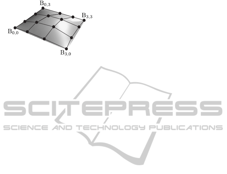
Figure 1: Bicubic B
´
ezier surface (n = m = 3).
where n is the degree of the Bernstein basis function.
These functions decide the extent to which a control
point controls the surface at a particular parametric
value t. Note that the first and last control points are
coincident with the end points of the curve, that is,
P(0) = B
0
and P(1) = B
n
.
The equation for a B
´
ezier curve can be also ex-
pressed in matrix form:
P(t) = [T ][N][G] (3)
where [T ] = [t
n
t
n−1
. . . t
1
t
0
], the geometry of the
curve is represented as [G]
T
= [B
0
B
1
. . . B
n
], and the
[N] matrix is defined by:
n
0
n
n
(−1)
n
n
1
n−1
n−1
(−1)
n−1
. . .
n
n
n−n
n−n
(−1)
0
. . . . . . . . . . . .
n
0
n
1
(−1)
1
n
1
n−1
0
(−1)
0
. . . 0
n
0
n
0
(−1)
0
0 . . . 0
For example, for n = 3 the matrix form is:
P(t) = [T ][N][G] =
[t
3
t
2
t
1
1]
−1 3 −3 1
3 −6 3 0
−3 3 0 0
1 0 0 0
B
0
B
1
B
2
B
3
(4)
Likewise, the shape of a (n, m)-degree B
´
ezier sur-
face is controlled by a set of control points through
the equation:
Q(u, v) =
n
∑
i=0
m
∑
j=0
B
i, j
J
n,i
(u)J
m, j
(v), 0 ≤ u, v ≤ 1 (5)
where J
n,i
(u) and J
m, j
(v) are the Bernstein basis func-
tions in the u and v parametric directions and B
i, j
are
the vertices of a polygonal control net. Again, the
number of control points in the u and v directions are
n+1 and m+1 respectively. As an example, Figure 1
shows a bi-cubic B
´
ezier surface, n = m = 3. In matrix
form, a B
´
ezier surface is given by:
Q(u, v) = [U][N][B][M]
T
[V ]
(6)
For the specific case of a bi-cubic B
´
ezier surface,
the matrix form is given by:
Q(u, v) = [u
3
u
2
u 1]
−1 3 −3 1
3 −6 3 0
−3 3 0 0
1 0 0 0
B
0,0
B
0,1
B
0,2
B
0,3
B
1,0
B
1,1
B
1,2
B
1,3
B
2,0
B
2,1
B
2,2
B
2,3
B
3,0
B
3,1
B
3,2
B
3,3
−1 3 −3 1
3 −6 3 0
−3 3 0 0
1 0 0 0
v
3
v
2
v
1
(7)
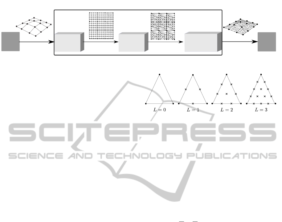
2.2 ESC Pipeline
Figure 2 schematically depicts the structure of this
proposal, whose goal is to reduce the number of trian-
gles of the final mesh while keeping the quality of the
resulting image. The proposed solution is based on
a 3-step programmable pipeline: first, a fixed tessel-
lation pattern is computed to guide the adaptive pro-
cedure for the patch; next, the new vertices obtained
from the first step are conditionally inserted by ap-
plying a set of heuristics consisting of tests local to
the triangle; finally, a specific scheme is employed to
reconstruct the mesh by processing the inserted ver-
tices.
The first step carries out a non recursive procedure
based on the utilization of a fixed tessellation pattern
to guide the tessellation. The level of resolution of
each object depends on the camera position and de-
termines the refinement degree of the surface. Once
the level of resolution is selected, only the positions
of the uniform tessellation pattern are evaluated for
their conditional insertion.
The tessellation patterns are employed to guide
the adaptive tessellation in such a way that the new
vertices can only be inserted in the candidate posi-
tions specified by the patterns. The second step de-
cides which candidate vertices are really inserted as a
result of a tessellation test (Local Test in Figure 2).
The evaluation of all samples of each surface takes
advantage of the constant result of [N][B][M]
T
for ev-
ery point on the surface and that the different control
points [B] are accessed only once, transforming the
Equation 6 in
Q(u, v) = [U][NBM][V ] 0 ≤ u, v ≤ 1
(8)
with [NBM] = [N][B][M]
T
, whereas the current DX11
tessellation proposal accesses to [B] and computes
[NBM] for each sample on the surface.
The last step of the adaptive tessellation algo-
rithms is the reconstruction of the mesh from the set
of vertices finally inserted; i.e. once the new vertices
FreeAdaptiveTessellationStrategyofBézierSurfaces
257
Tessellation
pattern
Local
test
Adaptive
tessellation
procedure
Tessellation ShaderVertex Shader Fragment Shader
Figure 2: Structure of the ESC tessellation proposal.
have been conditionally added, all the vertices (old
and new) have to be organized and connected to re-
construct the final mesh assuring no cracks or holes in
the result (Tessellation Procedure in Figure 2). The
meshing scheme is simple and a triangle strip is di-
rectly generated.
Regarding the test selected in this work to guide
the adaptive tessellation (Local test), a distance-based
heuristic was chosen. The objective of an adaptive
tessellation is to generate detailed structures only on
those areas where a high resolution is required while
keeping a coarse mesh in those areas where a higher
tessellation results only in a slight increment in the
quality of the final image. In (Concheiro et al., 2011)
a set of different tests local to the edges are presented.
Among them, the Distance test was selected for the
analysis and algorithms comparison performed in this
work.
This test analyzes the distance between the con-
trol mesh and the B
´
ezier surface. Specifically, the dis-
tance between a sampling point on the control mesh
and the corresponding point on the B
´
ezier surface is
evaluated. If the distance is small enough, the mesh
is considered a good approximation of the surface, so
no vertex is inserted. On the contrary, if the distance
is larger than a threshold a new vertex is introduced
as this will mean an increase in the quality of the final
image. The test is given by:
distance = [|V
S
−V
B
| > µ] (9)
where V
B
are the coordinates of the candidate vertex
V
B
on the B
´
ezier surface, V
S
are the coordinates of
the corresponding sampling point on the control mesh
and µ is a quality threshold selected on the basis of the
quality/timing requirements of the application. The
Distance test achieves good results in terms of quality
of the final mesh and has a reduced complexity and,
in this sense, is a good candidate to guide the adaptive
tessellation.
Figure 3: Triangle patterns for L = 0, 1, 2, 3.
3 ADAPTIVE TESSELLATION
STRATEGY
Although the versatility of ESC pipeline makes pos-
sible the use of different tessellation algorithms, the
strategy chosen in this work to perform an adaptive
tessellation of the input surfaces is described in this
section. The procedure starts by approximating the
surface with a coarse mesh and performing the adap-
tive tessellation of each coarse triangle. Specifically,
the control point mesh is partitioned into N
u
× N
v
cells of size
1
N
u
×
1
N
v
where two adjoining triangles
are generated per cell. The implementation employs
N
u
= N
v
= 3 cells so that eighteen coarse triangles are
generated per B
´
ezier patch. This number of triangles
is directly determined by the use of Bicubic surfaces.
A level of resolution L is assigned to the patch and
all triangles of the patch would be subdivided by em-
ploying a unique uniform tessellation pattern. Exam-
ples of tessellation patterns for different values of L
are depicted in Figure 3. The tests are only applied in
the candidate positions located in the original edges
of the coarse triangle. Finally, if a vertex is inserted
in the edge, the insertion is also performed along the
row in all the candidate positions inside the triangle.
An example of the vertex insertion procedure is
depicted in Figure 4. Figure 4a shows an example of
tessellation pattern for the adaptive proposals, respec-
tively. A single level of resolution L = 3 was selected
but three different tessellation level L = 1, L = 2 and
L = 3 can be applied to each edge. Figure 4b depicts
the result of tessellation once the insertion decisions
have been performed for the adaptive algorithms, re-
spectively. The test was applied on the original tri-
angle edges. As will be detailed in this section, this
GRAPP2014-InternationalConferenceonComputerGraphicsTheoryandApplications
258

1
2 3
4
5 6
7
8
9 10
11
Edge a
Edge c
Edge b
12
13
14
15
V
V
V
V
4
V V
V
V
V
V
V
V
V
V V
(a)
1
2
5 6
7
8
9
11
Edge a
Edge c
Edge b
12
13
15
V
V
V
V
V V
V
V
V
V
V
(b)
Figure 4: Adaptive tessellation (a) Adaptive pattern and (b)
Adaptive tessellation.
different test application procedure reduces the com-
plexity not only of the test phase but also of the mesh-
ing scheme employed to reconstruct the final triangle
mesh.
Once the insertion decisions have been taken a
meshing procedure to connect the vertices is per-
formed. Triangles are generated by connecting ver-
tices in two consecutive rows of vertices, larger trian-
gles connecting vertices in non-consecutive rows have
to be generated in those locations where vertices are
not inserted.
Once the subdivision tests are performed, the re-
sulting inserted vertices are organized into a set of
lists and the efficient management of this information
permits the reconstruction of the final mesh in a di-
rect way. A triangle strip is defined by a sorted list of
vertices:
T S =
{
v
1
, v
2
, ··· , v
Nt
}
where each triangle is defined by three sequential ver-
tices, with an overlap of two vertices between two
consecutive triangles. As an example the i − th tri-
angle is defined by:
4v
i
v
i+1
v
i+2
while the (i + 1) −th triangle is defined by:
4v
i+1
v
i+2
v
i+3
The basic idea of the representation and reconstruc-
tion algorithm is the organization of the resulting tri-
angles in rows and their representation as triangles
strips. The regular triangle strip structure is broken
only in those positions where no vertices are inserted.
(a) (b) (c)
Figure 5: Examples of semi adaptive tessellations (a) No
empty rows (b) Empty row, upper row with no missing ver-
tex (c) Empty row, upper row with a missing vertex.
This happens either in a position in the edge of the
coarse triangle or in a full row of vertices if both ver-
tices in the extreme positions are missing. For the
sake of clarity, we shall start by analyzing the case
when only one of the two extreme vertices of the row
are missing.
The methodology we propose is based on the uti-
lization of the TS structure that would be generated
with a non-adaptive tessellation as basis for the repre-
sentation. This T S list is updated with the utilization
of a Virtual Vertex (VV ) for the substitution of miss-
ing vertices. More specifically, each non-inserted ver-
tex on the edge of the triangle is substituted, in the
T S representation by the closest vertex located in the
same edge. A simple set of rules for updating the T S
structure when missing vertices appear are applied:
1. Missing vertex. If there is a non-inserted vertex in
a triangle edge, the VV is the vertex located on the
same edge and in the following row of vertices.
2. Group of missing vertices. If there is a group of
adjacent non-inserted vertices on a triangle edge,
each non-inserted vertex is replaced in the TS rep-
resentation by the nearest vertex on the edge. In
case of equidistant vertices, the vertex in the lower
row is selected.
3. Replicated vertices in the T S list. Once the miss-
ing vertices are replaced by virtual vertices, repli-
cated vertices can appear in the T S list. These
replicated vertices have to be eliminated; i.e., v
i
v
i
is substituted by v
i
.
4. Vertices from alternating rows. In the non-
adaptive partitioning, consecutive vertices in the
T S list belong to two rows of vertices. For the
adaptive proposal, when this regular structure is
broken a modification has to be performed. Let us
analyze a T S list with three consecutive vertices,
v
i
v
j
v
k
, where v
j
and v
k
come from the same row
of vertices. In this case the T S list is updated by
including a replicated version of v
i
in between. As
result the list of vertices becomes v
i
v
j
v
i
v
k
.
An example of application is depicted in Figure
5a. A non-adaptive tessellation would generate three
FreeAdaptiveTessellationStrategyofBézierSurfaces
259

rows of triangles, each one to be represented with at
T S list. The T S lists for the non-adaptive tessellation
are:
T S
1
= {v
2
v
1
v
3
}
T S
2
= {v
4
v
2
v
5
v
3
v
6
}
T S
3
= {v
7
v
4
v
8
v
5
v
9
v
6
v
10
}
(10)
As a result of the adaptive tessellation, the vertex v
6
is
not inserted. The T S lists are updated by the following
steps:
• The missing vertex v
6
is replaced by a virtual ver-
tex VV = v
10
. This is the closest vertex located in
the same triangle edge and in the following row
of vertices. As a result the T S
2
and T S
3
lists are
updated.
• The utilization of v
10
as virtual vertex in the T S
3
list generates a replicated vertex. According to
rule 3, the list T S
3
= {v
7
v
4
v
8
v
5
v
9
v
10
v
10
} be-
comes T S
3
= {v
7
v
4
v
8
v
5
v
9
v
10
}.
• With respect to the alternating rows prop-
erty and according to rule 4, the list
T S
3
= {v
7
v
4
v
8
v
5
v
9
v
10
} becomes
T S
3
= {v
7
v
4
v
8
v
5
v
9
v
5
v
10
}.
Finally the triangle strips for this example are:
T S
1
= {v
2
v
1
v
3
}
T S
2
= {v
4
v
2
v
5
v
3
v
10
}
T S
3
= {v
7
v
4
v
8
v
5
v
9
v
5
v
10
}
and the following triangles are generated:
T S
1
→ 4v
2
v
1
v
3
T S
2
→ 4v
4
v
2
v
5
4 v
2
v
5
v
3
4 v
5
v
3
v
10
T S
3
→ 4v
7
v
4
v
8
4 v
4
v
8
v
5
4 v
8
v
5
v
9
4 v
9
v
5
v
10
The methodology has to be extended to include
those situations in which both vertices in the extreme
positions of a row are missing. As the insertion de-
cisions are applied to the interior vertices in the same
row, this implies that a complete row of vertices is
missing. In this case fewer triangle strips are gener-
ated and a number of modifications have to be made
to the method explained above. The first step is to up-
date the T S lists of the non-adaptive case by identify-
ing the two T S lists affected and eliminating the first
one. After this the second list is updated by substitut-
ing the missing vertices by other vertices in the clos-
est non-empty row of vertices located above. More
specifically the substitution has to be performed by
adhering to the following rules:
1. Upper row with no missing vertices. If the row
above is complete, the vertices are directly em-
ployed to substitute the eliminated vertices in the
T S list. As the number of vacancies is larger
than the number of vertices, the vertices have to
(a) (b)
Figure 6: Models employed: (a) Teacup and (b) Elephant.
be replicated. To obtain a satisfactory tessella-
tion and to prevent the generation of large trian-
gles, the pattern of substitution/replication has to
be uniform.
2. Upper row with a missing vertex. If the row above
has a missing vertex, this location will be occu-
pied by a VV . The row of vertices is also em-
ployed to update the T S list under construction,
but a number of considerations have to be taken
into account for the VV . The vacancies are again
covered by the vertices in the row, but the VV ver-
tex can be employed only once; i.e., the VV can-
not be replicated.
Examples of application are depicted in Figures
5b and 5c. In these examples the row of vertices {v
4
,
v
5
, v
6
} has not been inserted. The T S lists generated
by the uniform tessellation (see Equation 10) have to
be updated. In this case lists T S
2
and T S
3
are affected
by the missing row and the list T S
2
is eliminated. List
T S
3
= {v
7
v
4
v
8
v
5
v
9
v
6
v
10
} has to be updated by
identifying the missing vertices (v
4
, v
5
and v
6
) and
replacing them with the list of vertices above. Specif-
ically, and for the example of Figure 5b, the vertices
to be employed are v
2
and v
3
. The number of vacan-
cies is larger, so the first two vacancies are covered
with vertex v
2
and the last one with vertex v
3
. The list
becomes T S
3
= {v
7
v
2
v
8
v
2
v
9
v
3
v
10
}.
Figure 5c shows an example where the row of ver-
tices to be employed has a missing vertex (v
2
). Fol-
lowing the methodology explained above, this vertex
is substituted by a virtual vertex, in this case by v
1
.
This virtual vertex is employed only once while ver-
tex v
3
is employed for the other two vacancies. So the
updated list is T S
3
= {v
7
v
1
v
8
v
3
v
9
v
3
v
10
}.
4 EXPERIMENTAL RESULTS
In this section, the results of the evaluation of ESC
pipeline are presented and analyzed. The adaptive
GRAPP2014-InternationalConferenceonComputerGraphicsTheoryandApplications
260

tessellation proposal is compared with the tessella-
tion implemented by the DirectX11 tessellation unit.
Specifically, we have used the code SimpleBezier11
included in the DirectX11 SDK to design an adaptive
solution (AdptTess) based on a distance test (as pre-
sented in Section 2.2) computed in the Hull Shader.
ESC proposal was coded in the Geometry Shader as
this makes it possible to implement a free tessellation
algorithm, even though it has the important constraint
of limiting the maximum number of new primitives
to be generated per input primitive to 1024 32-bit el-
ements.
Our algorithm was implemented with Microsoft’s
HLSL DirectX11, and the tests were run on an In-
tel Core 2 2.4 GHz with 2 GB of RAM and three
different GPUs: AMD/ATI Radeon 5870 (ATI 5870),
GPU with 1600 processing elements distributed in 20
SIMD processors, each one having 16 cores with 5-
way VLIW support; AMD/ATI Radeon 6970 (ATI
6970), with 1536 processing elements distributed in
24 SIMD processors, each one with 16 cores with 4-
way VLIW support; and Nvidia Geforce GTX 580
(Nvidia 580), GPU based on the Fermi architecture
that has 4 clusters, with 4 stream multiprocessor (SM)
per cluster and 32 stream processors per SM for a total
of 4× 4× 32 = 512 physical processing elements.
Two models were employed to evaluate the tessel-
lation (see Figure 6): Teacup and Elephant. These
models were used to build two test scenes, Teacups
and Elephants, that consist of replicated versions of
the models: 30, 100 and 10 models, respectively. To
check the performance of the implemented methods a
walk-through animation with the same movement of
the camera for the three scenes was performed. The
final images have a screen resolution of 1280 × 1024
pixels.
The next subsections focus on the analysis of the
experimental results in two different key points: the
analysis of the quality in the final image and the per-
formance in terms of frames per second.
4.1 Performance in Terms of Quality
As a starting point of the analysis of the results from
the tests, Table 1 presents the number of generated
primitives for each method. In this table the maxi-
mum resolution employed is L
max
= 3 (16 × 18 tri-
angles for each input surface). The second row indi-
cates the number of input B
´
ezier surfaces per scene.
The third row shows the number of triangles gener-
ated when a non-adaptive tessellation is applied. The
rest of the rows show the average number of triangles
generated by the adaptive proposal. The Distance test
was applied with two different thresholds on the basis
Table 1: Number of triangles generated (in thousands,
L
max
= 3) and number of input surfaces.
Teacups Elephants
Input Data 2600 8110
Non Adaptive 731.32 2280.94
Adaptive
High (93.62%) 684.67 (85.10%) 1941.03
Med (51.96%) 379.98 (50.68%) 1155.70
of a quality criteria: high or medium degree of tessel-
lation. The percentage of triangles obtained for each
case with regard to a non-adaptive strategy is shown
in parenthesis.
In our experiments, high quality meshes with no
cracks or holes are obtained. Obviously, the appli-
cation of the adaptive proposal gives rise to a reduc-
tion in the number of primitives generated, where the
decrement can be controlled by the adequate selection
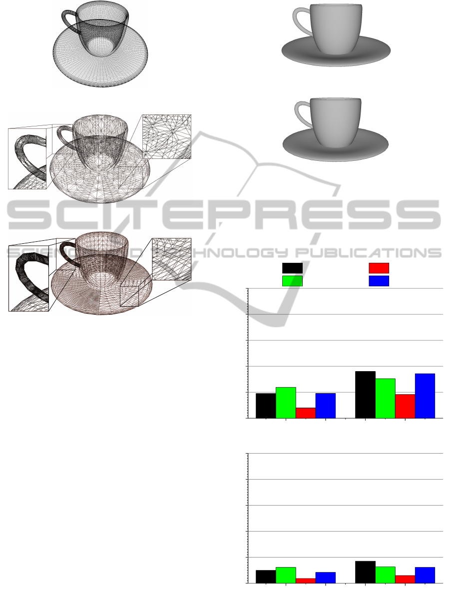
of the quality threshold applied. As an example of
the tessellation obtained, Figure 7 shows the result of
applying three different tessellation procedures to the
teacup model. Figure 7a depicts a non-adaptive tes-
sellation, with all the patches being uniformly subdi-
vided up to a resolution level determined by the point
of view, with a maximum refinement of L
max
= 3. Fig-
ure 7b shows the tessellation obtained by ESC, gen-
erating about a 50% of the triangles created with the
non-adaptive approach. Finally, the output obtained
by using AdptTess, configured to produce a similar
number of triangles than ESC, is depicted in Figure
7c.
As can be observed, significantly fewer primitives
are generated in the flat areas with the adaptive ap-
proximations, especially noticeable in the output from
ESC (see the detail being zoomed on the right of each
adaptive solution). In these flat areas the coarse mesh
is a good enough approximation to the B
´
ezier surface,
so introducing additional primitives does not result in
a higher quality of the image for the quality thresh-
old selected. Furthermore, as can be observed in the
zoomed detail on the left of the adaptive results, the
tessellation produced by ESC achieves a better ap-
proximation of the B
´
ezier surface, as geometric as-
pects are taken into account (distance-based heuristic)
in addition to the point of view information. Figure 8
shows a shaded version of the teacup model tessel-
lated by both adaptive approaches.
4.2 Performance in Terms of fps
Performance in terms of fps is another important as-
pect to be analyzed. Figure 9 shows the frames per
second (fps) with two different GPUs for an adap-
tive tessellation with a medium and high degree, as
FreeAdaptiveTessellationStrategyofBézierSurfaces
261
(a)
(b)
(c)
Figure 7: Examples of tessellation: (a) Non adaptive (b)
adaptive with ESC pipeline and (c) adaptive with AdptTess.
shown in Table 1. The column labeled as AdptT-
ess display the performance obtained by the Simple-
Bezier11 method implemented using the tessellation
unit. The tessellation factors have been selected to
generate a number of triangles similar to the obtained
Figure 9 shows that good performance results in
terms of frame rate (fps) were obtained, and a real-
time adaptive tessellation was achieved even for a
high number of triangles. Thus, for instance, the high
quality result of the Elephants scene is achieved with
a frame rate in our adaptive approach of 63.53 fps on
the ATI 6970, and 61.42 fps on the ATI 5870.
Broadly speaking, the frame rate achieved by ESC
is similar to AdptTess, and it is important to remark
that a software approximation of the algorithmic pro-
posal that ESC introduces has being used. It should
be pointed out that ESC demonstrates better compu-
tational exploitation than the tessellator-based alter-
natives, since one computing core (shader) is used for
each input primitive, instead of the one core per out-
put primitive ratio of the DirectX11 tessellator-based
proposals. As a result, an important feature of our
(a)
(b)
Figure 8: Shading comparison of the two adaptive ap-
proaches: (a) ESC pipeline and (b) AdptTess.
approach is the exploitation of the spatial coherence
of data, as shared common computations within the
0
100
200
300
400
500
FPS
AdaptTess Medium
ESC Adaptive Medium
AdaptTess High
ESC Adaptive High
ATI 5870 ATI 6970
(a) Teacups
0
100
200
300
400
500
FPS
ATI 5870 ATI 6970
(b) Elephants
Figure 9: Processing Speed in Frames per Second (L
max
=
3) (a) Teacups (b) Elephants.
GRAPP2014-InternationalConferenceonComputerGraphicsTheoryandApplications
262

same patch are computed only once and reused when
needed. This results in a better performance when the
number of primitives increases. Specifically, the re-
sults shown in Figure 9 say that, for the highest level
of tessellation, ESC is up to 2.25x faster on the ATI
5870 and up to 2.05x faster on the ATI 6970.
In summary, considering the good results ob-
tained, the flexibility of the adaptive proposals, the
exploitation of the locality and the prevention of re-
dundancy computations, our proposal is a good can-
didates to be integrated as a specific tessellation unit
in future graphics cards, as nowadays the existing tes-
sellation units included in current GPUs do not offer
the desirable adaptability.
5 CONCLUSIONS
This paper presents a proposal for the adaptive tes-
sellation of B
´
ezier surfaces on the GPU based on the
exploitation of the spatial coherence. The proposal do
not require the precomputation of any refinement pat-
tern, and the new vertices coordinates are computed
on-the-fly with a non recursive strategy. This permits
the exploitation of the vector computation capabilities
of current GPUs. The proposal uses a section of the
parametric map as input primitive.
This tessellation scheme reduces the divergence in
order to achieve an optimum utilization of the compu-
tational resources of the GPU; however, a remarkable
degree of adaptivity has been introduced. Hence, this
proposal processes considerably fewer triangles than
a non adaptive proposal.
The adaptive proposal is based on three main
strategies: the utilization of a fixed tessellation pat-
tern to guide the procedure, the utilization of a local
test to guide the tessellation decisions and an efficient
meshing procedure to reconstruct the resulting mesh.
Our proposal permits the application of multiple lev-
els of resolution to a B
´
ezier surface and exploits the
locality of the surface and, consequently, reducing the
number of shader invocations and, as a consequence,
the power consumption.
In addition to the good quality and performance
results, the flexibility of the adaptive proposal and the
simplicity of the computations involved could encour-
age the inclusion of more flexible tessellation units in
future graphics cards.
REFERENCES
Amresh, A. and F
¨
unfzig, C. (2010). Semi-uniform, 2-
Different Tessellation of Triangular Parametric Sur-
faces. In Proceedings of the 6th International Con-
ference on Advances in Visual Computing (ISVC’10).
Concheiro, R., Amor, M., and B
´
oo, M. (2010). Synthesis of
b
´
ezier surfaces. In GRAPP’10: International Confer-
ence on Computer Graphics Theory and Applications,
pages 110–115.
Concheiro, R., Amor, M., B
´
oo, M., and Doggett, M. (2011).
Dynamic and adaptive tessellation of bezier surfaces.
In GRAPP’11: International Conference on Com-
puter Graphics Theory and Applications, pages 100–
105.
Dyken, C., M., R., and Seland, J. (2009). Semi-uniform
Adaptive Patch Tessellation. Computer Graphics Fo-
rum, 28(8):2255–2263.
Eisenacher, C., Meyer, Q., and Loop, C. (2009). Real-time
View-dependent Rendering of Parametric Surfaces. In
Proceedings of the 2009 Symposium on Interactive 3D
Graphics and Games, pages 137–143.
Fisher, M., Fatahalian, K., Boulos, S., Akeley, K., Mark,
W. R., and Hanrahan, P. (2009). DiagSplit: Parallel,
Crack-free, Adaptive Tessellation for Micropolygon
Rendering. ACM Transactions on Graphics (TOG) -
Proceedings of ACM SIGGRAPH Asia 2009, 28(5).
Guthe, M., Bal
´
azs, A., and Klein, R. (2005). GPU-Based
Trimming and Tessellation of NURBS and T-Spline
Surfaces. ACM Trans. Graph., 24(3):1016–1023.
Munkberg, J., Hasselgren, J., and Akenine-M
¨
oller,
T. (2008). Non-uniform Fractional Tessella-
tion. In Proceedings of the 23rd ACM SIG-
GRAPH/EUROGRAPHICS Symposium on Graphics
Hardware.
Ni, T. and Casta
˜
no, I. (2009). Efficient Substitues for Sub-
division Surfaces. Exhibition Tech. SIGGRAPH’09
Course Notes, 2009.
NVIDIA (2008). NVIDIA CUDA Compute Unified Device
Architecture. Programming Guide.
Piegl, L. and Tiller, W. (1997). The NURBS Book. Springer.
Rogers, D. F. (2001). An Introduction to NURBS with His-
torical Perspective. Morgan Kaufmann.
Schwarz, M. and Stamminger, M. (2009). Fast GPU-based
Adaptive Tessellation with CUDA. Computer Graph-
ics Forum, 28(2):365–374.
Yeo, Y. I., Bin, L., and Peters, J. (2012). Efficient pixel-
accurate rendering of curved surfaces. In Proceedings
of the ACM SIGGRAPH Symposium on Interactive 3D
Graphics - i3D 2012, pages 165–174.
FreeAdaptiveTessellationStrategyofBézierSurfaces
263
