
Comparison of Different Color Spaces for Image Segmentation using
Graph-cut
Xi Wang
1
, Ronny H
¨
ansch
2
, Lizhuang Ma
1
and Olaf Hellwich
2
1
School of Electronic, Information and Electrical Engineering Shanghai Jiao Tong University,
800 Dong Chuan Road, 200240 Shanghai, P.R.China
2
Computer Vision and Remote Sensing Group, Technical University of Berlin, Marchstr. 23, 10587 Berlin, Germany
Keywords:
Graph-cut, Color Space, Image Segmentation.
Abstract:
Graph-cut optimization has been successfully applied in many image segmentation tasks. Within this frame-
work color information has been extensively used as a perceptual property of objects to segment the foreground
object from background. There are different representations of color in digital images, each with special char-
acteristics. Previous work on segmentation lacks a systematic study of which color space is better suited for
image segmentation. This work applies the Graph Cut algorithm for image segmentation based on five dif-
ferent, widespread color spaces and evaluates their performance on public benchmark datasets. Most of the
tested color spaces lead to similar results. Segmentations based on L*a*b* color space are of slightly higher
or similar quality as all the other methods. In contrast, RGB-based segmentations are mostly worse than a
segmentation based on any other tested color space.
1 INTRODUCTION
Color, as a visual perceptual property of objects, is
important in image coding, computer graphics, im-
age as well as video processing, and many more
computer vision tasks. Given the different needs of
those application areas, different methods are used
to represent color, each based on different mathe-
matical ideas, with different advantages and limita-
tions. Object segmentation has been deeply studied
since 1970s (R. Ohlander and Reddy, 1978) and is a
well-developed field within image processing. A seg-
mentation system derives a partition of a given image
into a set of (disjoint) regions. One particular case is
foreground-segmentation (FGS), where one or multi-
ple objects are considered as foreground and the rest
of the image is labeled as background. FGS plays an
important role in filmmaking as well as in photo and
video editing. It is also used as an intermediate result
for optical flow (T. Brox and Malik, 2009) and object
recognition (C.H. Gu and Malik, 2009).
As one of the fundamental properties of objects,
color has been used as important cue in several ob-
ject segmentation frameworks (P. Arbelaez and Ma-
lik, 2011; J. Shotton and Criminisi, 2009). Given the
range of needs of those methods as well as the var-
ious properties of existing color spaces, it is uncer-
tain which color space fits an individual segmentation
framework best and can lead to high performance.
During the last years graph-cut image segmenta-
tion has drawn a lot of attention and has for example
been applied to medical image analyzation (Boykov
and Jolly, 2001), color image segmentation (C. Rother
and Blake, 2004), and remote sensing image segmen-
tation (Sun and He, 2009). The Graph-Cut (GC) op-
timization framework (Boykov and Funka-Lea, 2006)
belongs to the category of segmentation approaches,
that are based on energy minimization. It allows the
usage of global as well as local knowledge and con-
straints, where other segmentation approaches con-
centrate on only one of them.
The aim of this work is to provide some insight
into the benefits and limitations of different color rep-
resentations, when included as local and global cue
into the GC segmentation framework as introduced in
(Boykov and Funka-Lea, 2006). For this goal color is
used as only cue, although other features like texture
are undoubtedly able to provide important informa-
tion for the segmentation process.
Segmentation is an ill-posed problem. The ac-
tual quality of any given segmentation can only be
judged with respect to the final application. For exam-
ple whether or not an object recognition system can
benefit from the segmentation. Nevertheless, a good
301
Wang X., Hänsch R., Ma L. and Hellwich O..
Comparison of Different Color Spaces for Image Segmentation using Graph-cut.
DOI: 10.5220/0004681603010308
In Proceedings of the 9th International Conference on Computer Vision Theory and Applications (VISAPP-2014), pages 301-308
ISBN: 978-989-758-003-1
Copyright
c
2014 SCITEPRESS (Science and Technology Publications, Lda.)

segmentation should inhibit some important proper-
ties. Most importantly, the set of object boundaries in
the image should be a subset of the segment bound-
aries, i.e. no segment covers both, fore- and back-
ground. In order to provide an objective measure of
performance in this comparative study, the GC seg-
mentation based on different color spaces is applied to
images from the Berkeley Segmentation Benchmark
(P. Arbelaez and Malik, 2011). In addition to a wide
range of images, this database provides manually la-
belled reference data. The results do not only depend
on the used color space, but also on the actual image
content. Thus, a second set of experiments is con-
ducted on the MSRC database (J. Shotton and Crimin-
isi, 2009), where individual objects within the images
are marked. The evaluation is carried out by compar-
ing the obtained segmentation results to the reference
data from those two benchmark datasets.
2 COLOR SPACE
There are many different color spaces proposed in the
literature, each with its own properties, advantages,
limitations, and areas of application. This work con-
centrates on five common examples, which are often
used in image processing tasks: RGB, HSV, L*a*b*,
L*u*v*, and the opponent color space. In order to
evaluate whether color information is meaningful at
all, a simple grayscale image representation is in-
cluded as sixth ”color” space.
Due to its simplicity the RGB color space is most
commonly used. It is represented by red (R), green
(G), and blue (B) chromaticities. The final color is
defined by the additive combination of those three pri-
mary colors.
The Hue, Saturation, and Value (HSV) color space
separates the intensity from the chromaticity and rep-
resents them independently. Hue describes the posi-
tion of the color in a 360
◦
spectrum. Saturation de-
scribes the pureness of the color: it measures the dif-
ference between the color and a grayscale value of
equal intensity. Value, as the third channel, is the
measurement of brightness.
The CIE L*a*b* and CIE L*u*v* spaces are se-
lected to represent a uniform color space. These two
color spaces are derived from the CIE XYZ color
space and attempt to produce a coordinate system in
which perceptual distances correspond to Euclidean
distances (Judd and Wyszecki, 1975). In CIE L*a*b*
color space, L* represents the lightness of color go-
ing from 0 (dark) to 100 (white), while the a* and
b* channels are the two chromatic components. The
first of these two (a*) represents the colors position
between red/magenta (+a) and green (-a). Similarly,
b* indicates its position between yellow (+b) and
blue (-b). In practice, their range goes from −128
to 127 with 256 levels. Similar to L*a*b*, the CIE
L*u*v* color space has one lightness channel and
two chrominance components referring to the same
chrominances. However, their transformation differs
from L*a*b*. The range for u* component goes from
−134 to 220 and −140 to 122 for v* component. The
advantage of L*u*v* color space is, that it has a more
linear transformation in the hue plane than L*a*b*
color space, however, these two are roughly equiva-
lent in representing a uniform perceptual color space.
The opponent color space has been claimed to
give better performance in several image processing
tasks (K. van de Sande and Snoek, 2008; Weijer and
Gevers, 2005). In this space, two channels, O
1
and
O
2
, are used to store the red-green and blue-yellow
opponent pairs, while the O
3
channel is equal to the
intensity channel in the HSV color space (K. van de
Sande and Snoek, 2008). Its transformation is given
by:
O
1
O
2
O
3
=
R−G
√
2
R+G−2B
√
6
R+G+B
√
3
(1)
3 GRAPH-CUT FRAMEWORK
The graph-cut framework proposed in (Boykov and
Funka-Lea, 2006) is used as the fundamental ob-
ject/background segmentation method in this work.
In the graph model, each pixel is considered as a node
and connected to its four neighbor nodes through
edges. Edges between pixel nodes are called n-links.
Additionally, there are two terminal nodes, S (source)
and T (sink), which represent object and background,
respectively. Each pixel node has two edges con-
nected to S and T , which are called t-links. All links
between two pixel nodes i and j are assigned with
nonnegative weights w
i j
. A cut through the graph is
defined by the removal of edges and produces a bipar-
tite graph in which there is no connected path from S
to T . The cost c(A, B) of this cut is calculated as:
c(A,B) =
∑
i∈A, j∈B
w
i j
(2)
where A and B correspond to the two disjoint sets of
nodes of the resulting bipartition. The min-cut/max-
flow algorithm finds the optimal cut with minimum
cost. This framework gives a pixel-precise segmenta-
tion. Figure 4(a)) shows a simple example for 3 ×3
VISAPP2014-InternationalConferenceonComputerVisionTheoryandApplications
302

S
T
cut
cut
Source
Sink
Figure 1: Segmentation example of a 3x3 image.
image, where the color information is used as cue to
assign the edge weights.
GC segmentation is semi-supervised and relies on
a small, manually labelled set of samples from fore-
and background. A novel user interface is used in this
work, which only requires a small fraction of the de-
sired object region to be marked. Figure 4(a)) gives
an example, where the red stroke marks the users se-
lection to indicate the foreground object. The system
then automatically estimates an approximate bound-
ing box for the selected foreground object. Back-
ground seeds are sampled uniformly distributed from
the outside-box area, while foreground seeds are se-
lected within the bounding box. It is assumed that
the region near the user-selected stroke has a higher
probability to belong to the foreground object. There-
fore, the foreground seeds are sampled according to a
Gaussian distribution along the red stroke. In Figure 4
background seeds are marked in green and foreground
seeds are marked in cyan.
The most crucial step of the whole framework
is the assignment of edge weights. Based on
the approach proposed in (Boykov and Funka-Lea,
2006), this work builds two Gaussian mixture mod-
els (GMM) from the sampled data of foreground ( f g)
and background (bg), respectively:
p(x|m) =
N
m
c
∑
i=1
α
m
i
·p(x|µ
m
i
Σ
m
i
), (3)
where m corresponds to either foreground ( f g) or
background (bg), N
m
c
is the number of components
of the corresponding GMM, and (α
m
i
,µ
m
i
,Σ
m
i
) are the
estimated parameters of the i-th component. They are
used to predict the probability that a certain pixel is
drawn from one of these two models. This probability
is assigned as weight to the corresponding t-links of
each node:
p(m|x) =
p(x|m) ·P(m)
p(x|f g) ·P( f g) + p(x|bg) ·P(bg)
, (4)
where m ∈ {f g,bg}. The prior probabilities are
set to P( f g) = P(bg) = 0.5 in this work. The weights
of the n-links w
i j
are assigned based on the difference
of color information between two pixels, i.e. the Eu-
clidean distance d(·) of the color vector of two adja-
cents pixels x
i
and x
j
:
w
i j
= exp
−
d(x
i
,x
j
)
σ
2
. (5)
4 EXPERIMENTAL RESULTS
4.1 Motivation and Introduction
In general, segmentation is an ill-posed and mostly a
rather subjective problem. The actual unbiased qual-
ity of a segmentation can only be judged in the context
of the final application, e.g. object recognition. The
second best way to evaluate a segmentation is to use
some kind of manually defined reference data. How-
ever, image segmentation by humans is highly sub-
jective, even if they agree on the kind (and number)
of foreground objects. If there is already some vari-
ation in the definition of the reference data, it cannot
be expected to obtain results by an (semi-)automatic
method, which are in full agreement with this ref-
erence data. Furthermore, not the actual quality of
the segmentation is tested, but the consistency with
the manual segmentation. The assumption, that those
two concepts are equivalent, might be invalid in many
applications. Nevertheless, two publicly available
benchmark datasets are used for evaluation in order
to provide a fair comparison.
It should be emphasized that the goal of this work
is not to achieve the best final segmentation, but to
compare the potential of different color representa-
tions. There is a high color similarity between fore-
ground and background in many images of the used
datasets. A good segmentation of those cases cannot
be achieved by color information alone. A realistic
segmentation method would include other cues. One
example are images of books or bikes. On the one
hand, these objects show a large within-class color
variation, which can be similar to the background. On
the other hand, they have a clearly defined shape or
structure.
In order to achieve an unbiased comparison of dif-
ferent color spaces, no other cue is used by the seg-
mentation framework, i.e. no texture or shape fea-
tures. Therefore, the results cannot be interpreted as
absolute accuracy measurements. The above men-
tioned facts cause a high quality variation in the com-
puted segmentations and the quality is expected to in-
ComparisonofDifferentColorSpacesforImageSegmentationusingGraph-cut
303

crease when other features are taken into account. In-
stead, the results are relative measures providing in-
formation which color representation is more suited
for image segmentation in general and specifically for
graph-cut segmentation.
4.2 Settings
The main object of each image is selected as fore-
ground, while the remainder is labelled as back-
ground. A manually marked stroke indicates the
area from which foreground samples are taken as de-
scribed above. In all experiments the same user input
is used, i.e. the same stroke marks the foreground ob-
ject.
In all the following experiments the same param-
eter settings are used. After transforming the given
color image into the color space under investigation,
the different image planes are normalized to the range
of zero and one. This allows to fix the scale factor
σ in Equation 5 to 0.2 for all color spaces. Both
GMMs consist of five components and describe the
joint probability in the respective three-dimensional
color space. The parameters of each GMM are esti-
mated by maximum likelihood from the samples of
each class, respectively.
4.3 Performance Measures
It is seldom the case in FGS that the foreground is
as large as the background. Mostly, one of those
two classes dominates the image. That is why the
main performance measurement used in this work to
compare different segmentations with respect to the
provided ground truth is the balanced accuracy (BA)
(K.H. Brodersen and Buhmann, 2010) given by Equa-
tion 6. It avoids biased performance estimates caused
by imbalanced data.
BA = (T PR + T NR)/2. (6)
The true positive rate T PR (sensitivity) gives the
percentage of correctly labelled foreground pixel and
the true negative rate T NR (specificity) gives the per-
centage of correctly labelled background pixel.
The authors of (D. Martin and Malik, 2001) ar-
gued, that an error measure, which compares two
given segmentations, should be robust regarding re-
finement, i.e. the error should be zero if one segment
in the first segmentation is a subset of a segment in
the second segmentation. If not, the error should be
inversely proportional to the overlap of the two seg-
ments. In (D. Martin and Malik, 2001) the authors
proposed the local refinement error as
E(S
1
,S
2
, p
i
) =
|R(S
1
, p
i
)\R(S
2
, p
i
)|
|R(S
1
, p
i
)|
, (7)
where R(S, p
i
) is the pixel set of the segment in
segmentation S, which contains pixel p
i
, \ denotes
set difference and |.| gives the cardinality of the set.
This error is not symmetric. It is used to define two
global error measures by forcing the refinement either
globally in one direction (Global Consistency Error,
GCE, Eq. 8), or allow for locally different directions
of refinement (Local Consistency Error, LCE, Eq. 9):
GCE =
1
n
min
(
n
∑
i=1
E(S
1
,S
2
, p
i
),
n
∑
i=1
E(S
2
,S
1
, p
i
)
)
(8)
LCE =
1
n
n
∑
i=1
(min{E(S
1
,S
2
, p
i
),E(S
2
,S
1
, p
i
)}) (9)
4.4 Experiment on BSDS500
The first set of tests are conducted on the Berkeley
segmentation dataset (BSDS500) benchmark (P. Ar-
belaez and Malik, 2011). This benchmark is origi-
nally not designed for FGS, but for general segmenta-
tion tasks. It consists of the 200 training and 100 test
images from the former BSDS300, and adds 200 new
test images, resulting in overall 500 images. GC seg-
mentation is independently applied to individual im-
ages and no learning from other images takes place.
That is why all 500 images are used.
For each of the images multiple segmentations are
provided, which were manually generated by differ-
ent humans. Those reference segmentations vary in
quality, i.e. in accuracy of segment boundaries. To
cast these general segmentations into the two class
problem of FGS, the most dominant object or group
of objects is selected as foreground, the remainder of
the image as background, and all segments in the ref-
erence data are accordingly assigned to one of those
two classes. Figure 2(a) shows one image example
from this dataset along with one of the reference seg-
mentations in Figure 2(b), as well as the two-class ref-
erence segmentation derived from it in Figure 2(c).
(a) (b) (c)
Figure 2: Image example from BSDS500. (a) original im-
age and (b) reference segmentation shown in edges. (c)
Two-class segmentation mask.
The above described segmentation framework is
applied to each of the 500 images independently. For
each image the mean value of the comparison of the
VISAPP2014-InternationalConferenceonComputerVisionTheoryandApplications
304

computed segmentation and the provided reference
segmentations is computed. Table 1 shows the av-
eraged mean values of each measurement for all 500
images in BSDS500. The best result is highlighted
through boldface type. ”Gray.” stands for grayscale
results and ”Opp.” stands for the opponent color
space.
Table 1: Average BA, TPR, TNR, GCE, and LCE for all
images in BSDS500.
Gray. RGB HSV
BA 0.6951 0.7997 0.8180
TPR 0.6544 0.7119 0.7033
TNR 0.7357 0.8874 0.9327
GCE 0.2590 0.1893 0.1601
LCE 0.2103 0.1475 0.1181
Opp. L*u*v* L*a*b*
BA 0.8152 0.8178 0.8163
TPR 0.6979 0.7000 0.6942
TNR 0.9324 0.9355 0.9383
GCE 0.1624 0.1612 0.1604
LCE 0.1202 0.1193 0.1178
The results clearly show the benefits of including
color information over only using grayscale images.
The usage of color, no matter in which representation,
increased the accuracy by more than 10%.
The differences between the individual color
spaces are considerably smaller. Among the tested
representations, the RGB space is least suited for seg-
mentation. Its accuracy is below 80% and thus more
than 1.5% smaller than that of all the others. The T PR
for RGB is 1% higher as for the other color spaces,
but that comes at the cost of including too much of
the background into the foreground segment, result-
ing in a much higher false-positive rate (or equiva-
lently lower true-negative rate).
The remaining four color spaces lead very simi-
lar results with respect to all five measurements. The
HSV color space gives the best overall accuracy and
global consistency error of all 500 images, and the
L*a*b* color space gives the lowest local consistency
error. The differences are small but significant, which
was tested by a two-tailed McNemar’s test with a con-
fidence level of 99%.
4.5 Experiment on MSRC
The BSDS500 dataset consists of unordered images
of highly variant content. During the corresponding
experiments it was noted that the segmentation results
differed not only between different color spaces, but
also depend on the particular image category. A color
space that performed well for some image categories
led to only inferior results for other types of images.
In order to investigate this subject further a second
benchmark dataset is used.
The MSRC dataset (J. Shotton and Criminisi,
2009) contains 591 images that are ordered into 20
different categories (e.g. animal, tree, building, etc.).
Within each category the content of the individual im-
ages is similar. This dataset is designed for object
recognition instead of segmentation. That is why it
provides corresponding labelled reference images ad-
ditionally to the image category label. The main ob-
ject (according to the image category) was selected as
foreground and the rest of the image as background.
Figure 3(a) shows an example together with the pro-
vided reference image in Figure 3(b) and the gener-
ated foreground-segmentation mask in Figure 3(c).
(a) (b) (c)
Figure 3: Image example from MSRC. (a) original image
and (b) label image. (c) Two-class segmentation mask.
Compared to the BSDS500 dataset, the images
of the MSRC dataset have a rather simple content.
The subjective segmentation is clearer, since the fore-
ground object can be easier defined. Most images
in MSRC have only one single object and the dif-
ference between background and foreground is clear.
However, the reference images provide only a coarse
object outline and are by far not as accurate as in
BSDS500.
Table 2 presents the values of the performance
measures obtained from the MSRC dataset averaged
over all images regardless of their category.
The general findings of the previous subsection
are confirmed by the results obtained by using the
MSRC dataset. The usage of color leads to an
large increase of accuracy compared to using only
grayscale images. The worse performance of the
RGB color space is even more obvious here. The
remaining color spaces show again very similar be-
haviour.
Table 3 illustrates the BA averaged over all im-
ages for each of the twenty available categories. Since
grayscale and RGB consistently performed worse,
they are omitted. The classes are ordered by the BA
value obtained by using L*a*b*, which is given in
the last column. The columns corresponding to the
ComparisonofDifferentColorSpacesforImageSegmentationusingGraph-cut
305

Table 2: Average BA, TPR, TNR, GCE, and LCE for all
images in MSRC.
Gray. RGB HSV
BA 0.7211 0.7961 0.8162
TPR 0.6436 0.6861 0.6990
TNR 0.7985 0.9061 0.9334
GCE 0.524 0.3481 0.2902
LCE 0.3911 0.2331 0.1732
Opp. L*u*v* L*a*b*
BA 0.8176 0.8179 0.8204
TPR 0.6973 0.6995 0.6992
TNR 0.9379 0.9362 0.9416
GCE 0.2786 0.2814 0.2732
LCE 0.1606 0.1643 0.1543
other three color spaces show the difference value to
the L*a*b* accuracy, where a negative value means
that the method performed worse. The two last lines
of the table count how often each color space outper-
formed all other color spaces (#best), and how often
it resulted in better segmentations than L*a*b* (#bet-
ter), respectively.
Table 3: Overall accuracy for 20 classes in MSRC.
Class HSV Opp. L*u*v* L*a*b*
Bike -1.72 -0.81 -1.26 71.84
Chair 0.05 -0.56 -0.8 75.89
Street -0.81 -1.62 0.11 77.44
Book 1.2 0 0.18 77.67
Car 0.19 1.08 0.56 78.58
Plane -1.16 -0.22 0.58 80.58
Boat -0.69 -0.33 1.21 80.63
Tree 0.75 0.53 -0.31 80.64
Sea -2.02 -0.69 -0.78 82.09
Animal 0.16 0.35 0.56 83.26
Flower 0.62 0.07 -0.49 83.52
Dog -0.22 -1.27 -0.19 83.55
Face 0.56 0.41 -0.08 83.83
Cow -1.02 -0.12 0.33 83.94
Cat -1.62 -1.97 -1.77 84.19
Bird -0.94 -1.8 -1.77 84.79
Sheep -0.1 1.07 -0.47 85.41
Building -1.44 -0.25 -0.33 86.14
Person -0.38 -0.06 -0.03 86.3
Sign -0.41 0.43 -0.41 90.85
#best 25% 15% 25% 35%
#better 35% 30% 35% -
The similarity of the individual accuracies of those
four color spaces are again notable. Also the slight su-
perior performance of L*a*b*, which outperformed
each other color space in approximately 70% of all
cases. It resulted in better segmentation than any other
color space in still 35% of the cases. If L*a*b* is out-
performed by another color space, then the difference
in performance is on average smaller than if it led to
better results. Thus, L*a*b* gives better results on
average, although the difference is only small.
The relative ordering of the individual categories
is also notable. All color spaces show the worst
performance with “hard” classes like “Bike” and
“Chair”, which consists of many fine structures with
considerable gaps in between. These gaps are in-
cluded into the object area within the reference data,
which leads to a mixture of fore- and background
samples within the GC framework. The best per-
formance is achieved for “easy” categories like the
“Sign” class. These objects have clear boundaries,
show only a limited set of colors which are designed
to be distinct from the background, and have no note-
able 3D structure which could lead to color changes
due to inhomogeneous lighting. Apart from only a
few exceptions this relative ordering is consistent with
respect to the different color spaces.
Additional to the relative ordering of the classes
based on the accuracy of the corresponding segmen-
tation, they are also grouped into coarser semantic
categories. One example is the “Vehicle” category,
which consists of “Car”, “Plane”, and “Boat”. An-
other even larger group consists of every animal class
within the dataset (but includes “Flower” and “Face”
as well). There are “radiometric” groups as well,
which consists of object categories that show simi-
lar foreground-background statistics. One example is
the aforementioned problem caused by the fine struc-
tures of chairs and bikes, which lead to a mixture of
foreground and background samples. Another exam-
ple are “Tree” and “Sea” categories. Images in those
classes consists of a rather large foreground object,
which has a very similar color to a huge part of the
background (lawn in the tree class and the blue sky in
the sea class).
Table 3 shows, that the segmentation accuracy in-
deed depends on the object category, but the differ-
ences are only small, i.e. less than 2% in all cases.
There is no single best color space, although L*a*b*
leads to slightly better results on average. The rela-
tive performance of different color spaces is not con-
sistent for any of the groups discussed above. L*a*b*
seems to be able to deal better with animal categories,
where it is outperformed in three out of six cases, two
times by the very similar L*u*v* color space. In gen-
eral the results of these two color spaces are close to
each other most of the time. The largest difference
is caused by the bird and cat classes, where L*a*b*
color space demonstrates a better ability to deal with
illumination variance. Figure 4 illustrates segmenta-
VISAPP2014-InternationalConferenceonComputerVisionTheoryandApplications
306
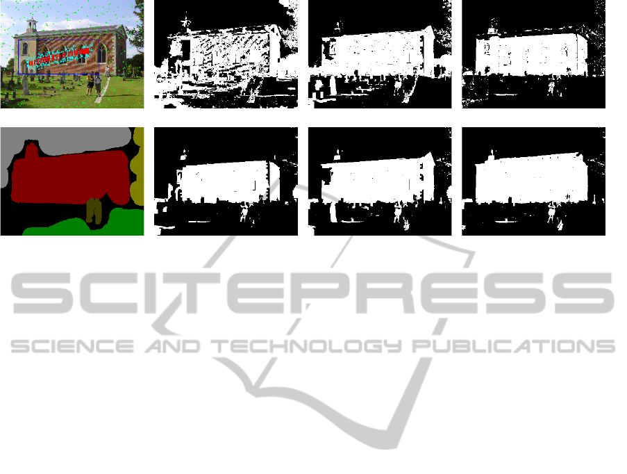
(a) (b) (c) (d)
(e) (f) (g) (h)
Figure 4: Segmentation results for a house image. (a) Original image with random selected sample seeds. (e) Reference
image. (b) (c) (d) (f) (g) (h) are the segmentation results in Grayscale, RGB, HSV, opponent color space, L*u*v* and L*a*b*
color spaces respectively. White area indicates the selected foreground.
tion results of a “Building” image. The L*a*b* color
space gives the best result. It is robust to illumination
changes and thus able to segment the shadow area of
the house correctly. RGB, opponent color space and
L*u*v* failed to correctly segment the left part of the
building. The roof is segmented as part of the back-
ground in all the color spaces except L*a*b*.
4.6 Summary
The experiments clearly show that color is an impor-
tant and very descriptive property of objects in im-
ages. Segmentation methods like GC greatly benefit
from the usage of color instead of relying on gray-
scale images alone.
The results of all color spaces are close to each
other. No color space actually failed to provide a
meaningful segmentation. The results from both test
sets suggest that L*a*b* is best suited for foreground
segmentation. The intrinsic color component is bet-
ter presented in L*a*b* color space. Therefore, it can
deal better with shadow and other lighting changes.
The difference to the second best color space is only
small, but significant. The second best choice is either
L*u*v* or HSV. RGB is the least suited color space
in the tested FGS scenario.
The performance of the segmentation method
does depend on the object category, in particular on
relative statistics of fore- and background. Again,
L*a*b* shows best results on average, but is outper-
formed by any of the other color spaces in 65% of the
cases. However, the winning method is not consis-
tently distributed over the other color spaces.
It should be noted, that the tested segmentation
framework strongly depends on the Gaussian assump-
tion. Gaussian mixture models are used to estimate
the color model of fore- and background and the dif-
ference of two adjacent color pixel is measured by the
Euclidean distance. L*a*b* and L*u*v* are designed
so that the perceptual difference of individual colors
is proportional to the distance in the corresponding
three-dimensional vector space. This assumption is
problematic for the HSV color space, where the hue
values (as main component representing color) lie on
a ring. It is also well known, that the perceptual dif-
ference of RGB colors does not correspond to the Eu-
clidean distance within the RGB vector space. Nev-
ertheless the Euclidean distance is commonly used
and it is not a trivial task to design distance measures
which better represent perceptual differences in those
color spaces.
5 CONCLUSIONS AND FUTURE
WORK
This paper provides a first comparative study of dif-
ferent color spaces in the context of image segmenta-
tion based on graph-cut. A GMM-based color model
is automatically build to assign weights to the t-links,
while an exponential transform of the Euclidean dis-
tance is used as n-links weight.
An easy-to-use user interface is provided to in-
dicate the foreground object. Experiments are con-
ducted in six color spaces: Grayscale, RGB, HSV,
opponent color space, L*u*v*, and L*a*b*. The seg-
mentation accuracy estimated over nearly 1100 dif-
ferent images shows on the one hand that there is
ComparisonofDifferentColorSpacesforImageSegmentationusingGraph-cut
307

no overall best color space. The quality depends not
only on the color space, but is as well data depen-
dent, i.e. varies for different object classes. On the
other hand L*a*b* shows a strong tendency to lead to
good results, which compare favorably even in cases
where other color spaces show a slightly higher per-
formance.
The objective of this work is to study the impact
of five different, commonly used color spaces on seg-
mentation obtained by Graph-Cut. Future work will
extend the current work mainly in four directions:
Firstly, a larger range of color spaces will be included
for comparison in order to provide a more exhaustive
study on the topic and to improve the preliminary con-
clusions given in this work. Secondly, experiments
will also be conducted using other semi-supervised
image segmentation methods, such as fuzzy informa-
tion fusion algorithm (Valet et al., 2001), decision
forests (J. Shotton and Criminisi, 2009) and so on.
Thirdly, a final segmentation approach should not be
based on color alone. Instead other cues should be
exploited as well. Texture will be included into the
segmentation framework in order to study the inter-
play between those two complementary cues. For this
purpose textons (Julesz, 1986) will be used to extract
texture information, while the radiometric properties
are captured by different color models. Fourthly, a
more thoroughly analysis on the interdependence of
different color spaces and image/object category on
the segmentation results will be carried out.
ACKNOWLEDGEMENTS
This work is funded in part by National Natural Sci-
ence Foundation of China No. 61133009 and No.
61073089.
REFERENCES
Boykov, Y. and Funka-Lea, G. (2006). Graph cuts and ef-
ficient nd image segmentation. International Journal
of Computer Vision, 70(2):109–131.
Boykov, Y. Y. and Jolly, M. P. (2001). Interactive graph
cuts for optimal boundary and region segmentation of
objects in n-d images. 8th IEEE International Confer-
ence on Computer Vision, 1:105–112.
C. Rother, V. K. and Blake, A. (2004). Grabcut: Interactive
foreground extraction using iterated graph cuts. ACM
Transactions on Graphics (TOG), 23(3):309–314.
C.H. Gu, J. J. Lim, P. A. and Malik, J. (2009). Recogni-
tion using regions. In IEEE Conference on Computer
Vision and Pattern Recognition, CVPR, pages 1030–
1037.
D. Martin, C. Fowlkes, D. T. and Malik, J. (2001). A
database of human segmented natural images and its
application to evaluating segmentation algorithms and
measuring ecological statistics. In Eighth IEEE Inter-
national Conference on Computer Vision, volume 2,
pages 416–423.
J. Shotton, J. Winn, C. R. and Criminisi, A. (2009). Tex-
tonboost for image understanding: Multi-class object
recognition and segmentation by jointly modeling tex-
ture, layout, and context. International Journal of
Computer Vision, 81(1):2–23.
Judd, D. B. and Wyszecki, G. (1975). Color In Business.
John Wiley and Sons, London, 2nd edition.
Julesz, B. (1986). Texton gradients: The texton theory re-
visited. Biological Cybernetics, 54(4-5):245–251.
K. van de Sande, T. G. and Snoek, C. G. (2008). Color de-
scriptors for object category recognition. In In Euro-
pean Conference on Color in Graphics, Imaging and
Vision, volume 2, pages 378–381.
K.H. Brodersen, C.S. Ong, K. S. and Buhmann, J. (2010).
The balanced accuracy and its posterior distribution.
In Proceedings of the 20th International Conference
on Pattern Recognition, pages 3121–3124.
P. Arbelaez, M. Maire, C. F. and Malik, J. (2011). Contour
detection and hierarchical image segmentation. IEEE
Transactions on Pattern Analysis and Machine Intel-
ligence, 33(5):898–916.
R. Ohlander, K. P. and Reddy, D. R. (1978). Picture seg-
mentation using a recursive region splitting method.
Computer Graphics and Image Processing, 8(3):313–
333.
Sun, F. and He, J. P. (2009). The remote-sensing image seg-
mentation using textons in the normalized cuts frame-
work. In International Conference on Mechatronics
and Automation (ICMA), pages 9–12.
T. Brox, C. B. and Malik, J. (2009). Large displacement
optical flow. IEEE Conference on Computer Vision
and Pattern Recognition (CVPR), 41(48):20–25.
Valet, L., Mauris, G., Bolon, P., and Keskes, N. (2001).
Seismic image segmentation by fuzzy fusion of at-
tributes. Instrumentation and Measurement, IEEE
Transactions on, 50(4):1014–1018.
Weijer, J. V. D. and Gevers, T. (2005). Boosting saliency
in color image features. In In Computer Vision and
Pattern Recognition (CVPR), volume 1, pages 365–
372.
VISAPP2014-InternationalConferenceonComputerVisionTheoryandApplications
308
