
Kernel-based Adaptive Image Sampling
Jianxiong Liu, Christos Bouganis and Peter Y. K. Cheung
Department of Electrical and Electronic Engineering, Imperial College London, London, U.K.
Keywords:
Progressive, Image Sampling, Kernel Regression.
Abstract:
This paper presents an adaptive progressive image acquisition algorithm based on the concept of kernel con-
struction. The algorithm takes the conventional route of blind progressive sampling to sample and reconstruct
the ground truth image in an iterative manner. During each iteration, an equivalent kernel is built for each
unsampled pixel to capture the spatial structure of its local neighborhood. The kernel is normalized by the es-
timated sample strength in the local area and used as the projection of the influence of this unsampled pixel to
the consequent sampling procedure. The sampling priority of a candidate unsampled pixel is the sum of such
projections from other unsampled pixels in the local area. Pixel locations with the highest priority are sampled
in the next iteration. The algorithm does not require to pre-process or compress the ground truth image and
therefore can be used in various situations where such procedure is not possible. The experiments show that
the proposed algorithm is able to capture the local structure of images to achieve a better reconstruction quality
than that of the existing methods.
1 INTRODUCTION
Progressive Image Transmission (PIT) is a family of
methods that aims to make efficient use of the limited
bandwidth to transmit large image data (Tzou, 1986).
The system can stop at any time during the transmis-
sion and still be able to reconstruct an approximation
to the ground truth image. Algorithms designed for
PIT are able to rearrange the order of transmission so
that significant data is transmitted first. The signifi-
cance is determined by the application and it is most
commonly defined as the potential of bringing a high
improvement to the quality of reconstructed image.
Early designs of PIT algorithm include the Bit-
Plane method (BPM) which is the basic technique cat-
egorized as one of the spatial domain techniques by
the author (Tzou, 1986). Chang and Shiue (Chang
et al., 1999) proposed an improved method based
on BPM but all BPM-based algorithms require high
transmission bandwidth. Later, various other algo-
rithms based on vector quantization were proposed,
including side-match PIT scheme (Chen and Chang,
1997) and the selective PIT (Jiang et al., 1997). There
are also techniques based on point sampling and tri-
angulation. Siddavatam Rajesh proposed a progres-
sive image sampling technique inspired by the lift-
ing scheme of wavelet generation and the sampled
pixels are used in non-uniform B-Spline to approx-
imate the ground truth image (Rajesh et al., 2007).
Demaret developed a similar method by using adap-
tive thinning algorithm (Demaret et al., 2006) to iden-
tify the significant pixels. Verma et al. proposed to
use gradient information as significance of pixels and
use linear bivariate splines to reconstruct(Verma et al.,
2010). There are also techniques based on trans-
form domain. The Discrete Cosine Transform (DCT)
and Discrete Wavelet Transform (DWT) were used in
many techniques to transform the image to frequency
domain. Such transforms are used in the popular
JPEG and JPEG2000 standards (Skodras et al., 2001)
(Chang et al., 2008) (Chang and Lu, 2006) as the pre-
processing stage of the compression process. Based
on the transformed image, further discussions about
the progressive transmission of the coefficients were
made . The coefficients can be transmitted progres-
sively in a hierarchical way, or in more complicated
manner such as that proposed by Shapiro (Embed-
ded Zerotree Wavelet coder (Shapiro, 1993)) or later
by Amir Said (Set Partitioning in Hierarchical Trees
(Said and Pearlman, 1996)).
Despite of the many techniques developed in the
past decade, few of them can operate without pre-
processing the image. Most of the techniques require
to analyze the ground truth image first to find out an
optimized order of transmitting the data. However in
practice many applications, such as graphics render-
25
Liu J., Bouganis C. and Cheung P..
Kernel-based Adaptive Image Sampling.
DOI: 10.5220/0004653100250032
In Proceedings of the 9th International Conference on Computer Vision Theory and Applications (VISAPP-2014), pages 25-32
ISBN: 978-989-758-003-1
Copyright
c
2014 SCITEPRESS (Science and Technology Publications, Lda.)

ing and range sampling, do not have the ground truth
image readily available – sampling can only be done
in a blind way. In such applications, it is often ex-
pensive to sample a pixel and therefore the concept of
PIT also applies well. Non-uniform stochastic point
sampling is often used in these situations where the
statistics of the image to sample is unknown. Eldar et
al. (Eldar et al., 1997) proposed the Farthest Point
Strategy (FPS) as an stochastic model that ensures
maximum sample distance. He also introduced the
data adaptive version of FPS (AFPS) to benefit from
previously sampled pixels. Later, Devir successfully
applied this idea in range sampling system and gen-
eralized it to accommodate grid sampling (Devir and
Lindenbaum, 2007).
This paper proposes a progressive image sampling
technique that does not require pre-processing of the
ground truth image. The proposed technique sam-
ples an amount of pixels at each iteration, based on
estimated pixel priority from previous samples. The
pixel priority is modeled by building equivalent ker-
nels which adapt to the local embedded structure of
the image. The rest of the paper is arranged as fol-
lows: In section II we will generalize the problem
of progressive point sampling; in section III we will
explain the details of the proposed technique; finally
experimental results are listed and discussed in Sec-
tion IV, showing the improved ability of the system to
identify and sample significant pixels at early stage,
resulting in an improved reconstruction quality.
2 GENERALIZED FRAMEWORK
OF POINT SAMPLING
In situations where the ground truth image is not read-
ily available, stochastic point sampling is suggested to
have advantages over uniform sampling (Eldar et al.,
1997). An approximation to the image can be recon-
structed from the non-uniformly sampled pixels by
interpolation based on triangulation technique. Con-
ventional point sampling algorithms are designed to
generate sampling patterns ensuring both randomness
and maximum distance. The randomness is intro-
duced to reduce the effect of potential aliasing while
the maximum distance is based on the basic assump-
tion of signal continuity. On top of that, the sampling
process can be refined iteratively to better adapt to the
sampled data. As proposed by Eldar et al., the sam-
pling process can be data adaptive by modeling the
priority score of each candidate unsampled pixel to
be the product of its Euclidean distance to the near-
est sampled pixel and its estimated local bandwidth.
To ensure the maximum distance, candidates in AFPS
are always the Voronoi vertices of the triangulation
formed by the already sampled pixels. As shown in
Fig.1, the candidate unsampled pixel i has a priority
score determined by the three vertices of the enclos-
ing triangle (Eldar et al., 1997):
f (x
i
) =
k
x
i
−x
s
1
k
2
∗max
k6=l
(B
min
(x
s
k
,x
s
l
)) (1)
Figure 1: AFPS example: black dots are already sampled
pixels.
This priority score was extended from Voronoi
vertices to all unsampled pixels in (Devir and Linden-
baum, 2007) to allow sampling on regular grid:
f (x
i
) = min
k=1,2,3
(
x
i
−x
s
k
2
) ∗log(1 +
ˆ
σ
2
) (2)
Where
ˆ
σ is the weighted local variance of point x
i
.
We further extend the concept to a more general
form for point sampling as the product of distance
term and variance term:
f (x
i
) = d
x
i
,P
∗v
i
P : sampled pixel locations (3)
Where x
i
is the coordinate vector of a candidate un-
sampled pixel, and d
x
i
,P
measures the likelihood of
determining pixel x
i
with existing samples. This
distance therefore includes but is not limited to Eu-
clidean distance. The term v
i
is the estimated vari-
ance of pixel x
i
. In the next section, we will explain
in detail how to model the two terms using equivalent
kernels, to better capture the embedded spatial struc-
ture of natural images.
3 ADAPTIVE SAMPLING WITH
EQUIVALENT KERNEL
In (Takeda et al., 2007), Takeda et al. generalized the
use of kernels in image regression. Covering sim-
ilar ideas such as the popular Bilateral Filter, they
built a generalized framework of using the concept
of kernel in regression with non-uniformly sampled
pixels, as well as filtering the rough estimation to im-
prove the image quality. In particular, they proposed
to refine a rough estimation by applying the steerable
VISAPP2014-InternationalConferenceonComputerVisionTheoryandApplications
26

Figure 2: Effects of applying the steering matrix C
i
= γ
i
U
θ
i
Λ
i
U
T
θ
i
; the shape of the kernel is changed to reflect the local image
structure (Takeda et al., 2007).
kernel, which showed the capability of kernel-based
method to represent the spatial relationship between
pixel pairs.
The formulation of kernel regression comes natu-
rally from the local expansion of a universal regres-
sion function defined around sampled points. Based
on the assumption of local smoothness to some order
N, a relationship between a given sample and the pixel
to be estimated is established. And the final estimate
of the unknown pixel is formulated as a weighted sum
of sampled pixels, where the weights (equivalent ker-
nels) are determined by the geometrical and statistical
correlation between a sample and the unknown pixel.
In this work however, the similar concept is used
in modelling not for the regression but the sampling
priority of unknown pixels at each sampling iteration.
This is based on the fact that the sampling process
serves the regression or interpolation process which
eventually reconstructs the image. Therefore the sta-
tistical correlation between pixels derived for the ker-
nel regression technique also applies and can guide
the sampling process to prepare a more suitable sam-
pling pattern leading to a higher reconstruction confi-
dence.
3.1 Modeling the Variance Term
The core idea of steerable kernel, as is used in im-
age regression, is its ability to identify the local spa-
tial relationship between pixel locations. The con-
struction of steerable kernel requires gradient infor-
mation of the local area, which can be computed by
applying Sobel operators on the rough estimate from
previously sampled pixels. Although gradient infor-
mation computed in this way is an approximation of
the ground truth, it can still provide guidance to build
steerable kernels. Without losing generality, here we
make two assumptions:
1. A1: Assume that around each candidate unsam-
pled pixel, the samples in its neighbourhod are
dense enough to provide information for the con-
structing of a stable steerable kernel;
2. A2: Assume that each unsampled pixel that is
going to be interpolated after sampling steps, is
of same importance to the reduction of the Mean
Squared Error of the reconstructed image.
It is worth noting that A1 is always an approxima-
tion in practice, although it serves as the foundation to
the construction of kernels in related techniques. For
kernel regression, A1 directly impacts the reconstruc-
tion quality of the image. However for the purpose of
point sampling as this work does, the requirement is
more relaxed because the model is continuously be-
ing refined and A1 becomes more accurate during the
course.
Instead of directly modeling the variance of an
unsampled pixel, we first model the relationship be-
tween the pixel in question or in other words, project
its requirement of information to its neighborhood. If
we set the order N = 0, i.e. Nadaraya-Watson Esti-
mator (NWE), the classic kernel regression sees the
kernel centered on an unsampled pixel x to be:
ˆ
K(x
i
) =
K
h
(x
i
−x)
∑
x
i
K
h
(x
i
−x)
, K
h
(t) =
1
h
K(
t
h
), x
i
∈P (4)
Where h is the global smoothing parameter and
P is the collection of samples in the local area. The
regression is essentially a weighted sum of the local
samples and it reflects the basic continuity assumption
behind image interpolation. To model for the sam-
pling process, notice that this kernel function can also
be computed on Q, the collection of unsampled pix-
els, to form a complete kernel in the local area. The
weights on unsampled pixels, indicated by this kernel,
can be regarded as their potential correlation with x
i
.
To take into consideration of the local spatial
structure, the global smoothing parameter is modified
Kernel-basedAdaptiveImageSampling
27

Figure 3: Examples of equivalent kernel. The kernel shows a strong correlation among pixels along estimated edges; on flat
surface the kernel is more spread out, reflecting a more unbiased connection with neighboring pixels; on corner regions, the
kernel is very centered due to a complex embedded structure. The accumulated kernel value on the candidate unsampled pixel
in (a), projected from neighbouring samples, reflects the variance or freedom of this pixel during the reconstruction process.
to local smoothing matrix H
steer
x
= h ∗C
−
1
2
x
. Where
the covariance matrix C
x
can be computed by:
C
x
= γ
x
U
θ
x
Λ
x
U
T
θ
x
(5)
U
θ
x
=
cosθ
x
sinθ
x
−sinθ
x
cosθ
x
(6)
Λ
x
=
σ
x
0
0 σ
−1
x
(7)
The parameter set (σ
x
,θ
x
,γ
x
) is computed from
singular value decomposition of the matrix of local
gradients. If z
x
1
(·) and z
x
2
(·) are first derivatives of
the grayscale value along x
1
and x
2
directions respec-
tively, then the decomposition of the gradient matrix
in the neighborhood is:
.
.
.
.
.
.
z
x
1
(x
j
) z
x
2
(x
j
)
.
.
.
.
.
.
= U
x
S
x
V
T
x
, x
j
∈ P ∪Q (8)
The rotation angle θ
x
is computed from v
2
=
ν
1
,ν
2
, the second column of the orthogonal matrix
V
x
.
θ
x
= arctan(
ν
1
ν
2
) (9)
The elongation parameter is the ratio of the energy
in the two dominant directions, indicated by the two
diagonal elements of S
x
: σ
x
= s
1
/s
2
. The scaling pa-
rameter γ
x
is determined by the geometric mean of the
energy normalized by the number of pixels M in the
neighbourhood: γ
x
=
√
s
1
s
2
/M. The effect of apply-
ing the steering matrix on the kernel function is shown
in Fig.2.
The final equivalent kernel constructed with the
steerable smoothing matrix in the local area is then
defined as:
ˆ
K
x
(x
i
) =
K
H
steer
x
(x
i
−x)
∑
x
i
K
H
steer
x
(x
i
−x)
, x
i
∈ P ∪Q (10)
K
H
steer
x
(x
i
−x) =
p
det(C
x
)
2πh
2
exp
−
(x
i
−x)
T
C
x
(x
i
−x)
2h
2
(11)
The equivalent kernel constructed in this way is
regarded as an “ideal kernel” that describes the lo-
cal structure of the image. It is centered on each un-
sampled pixel and covers a local area around it. It is
computed from local statistics (A1), and is normal-
ized to have a sum of 1 to reflect the same amount of
influence each unsample pixel is able to project to its
neighborhood (A2). If x
i
∈Q, a large
ˆ
K
x
(x
i
) indicates
that as a candidate unsampled pixel x
i
being sampled
next will make x more likely to be interpolated accu-
rately due to its high correlation with x
i
. The variance
term in (3) is therefore the sum of all the pair-wise
relationship between a candidate unsampled pixel x
i
and other unsampled pixels in its neighborhood:
v(x
i
) =
∑
x∈Q
ˆ
K
x
(x
i
), x
i
∈ Q
global
(12)
An example of accumulating for the variance term
is given in Fig.3. In this example, the candidate un-
sampled pixel in the middle has an accumulated vari-
ance score from other unsampled pixels in the neigh-
borhood, all of which have their own equivalent ker-
nels centered on them. The candidate can be any
unsampled pixel, or certain pixel locations selected
by other algorithms, such as those that happen to be
Voronoi vertices at the same time.
Given all the unsampled pixels x ∈ Q to interpo-
late, a higher variance term v(x
i
) indicates that sam-
pling x
i
is likely to reduce a large amount of collec-
tive variance of its neighborhood, therefore is more
capable of stabilizing the local interpolation and has a
bigger impact to improving the image quality.
VISAPP2014-InternationalConferenceonComputerVisionTheoryandApplications
28
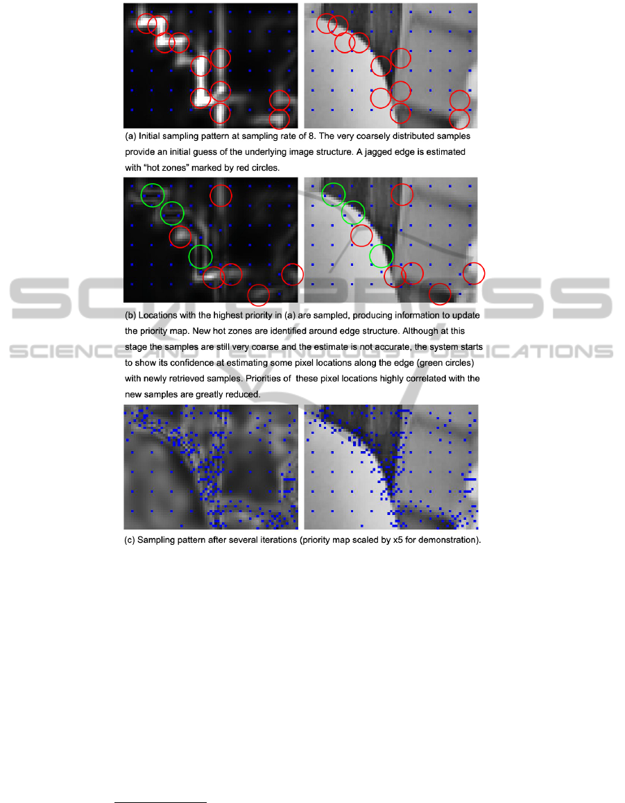
Figure 4: Example of the sample process. Blue dots are sampled locations; graphs on the left hand side are priority maps in
grayscale, showing candidate pixel locations with higher priority score f (x
i
) in brighter dots; pictures on the right hand side
are the original image patch.
3.2 Modeling the Distance Term
Although unsampled, some pixels are more deter-
mined than others because within its neighborhood,
more highly correlated pixels have already been sam-
pled. The distance term is therefore to compensate
for this effect. To measure the likelihood of determin-
ing pixel x with already sampled pixels, we define the
sample strength within its neighborhood to be:
l
P
(x) =
∑
x
i
∈P
ˆ
K
x
(x
i
)
max
x
i
∈P
(
ˆ
K
x
(x
i
))
(13)
It is closely related to the sample density discussed
in (Takeda et al., 2007), but is normalized by the high-
est value of the equivalent kernel, to reflect that the
most related pixels within the neighborhood (often the
closest ones) should have the maximum correlation
value of 1. This is also based on the basic continuity
assumption of natural images. By virtue of equivalent
kernel, the sample strength takes into account both the
spatial distance and the embedded image structure. A
higher sample strength will reduce the total influence
that an unsampled pixel is able to project to its neigh-
borhood. The distance term of x is therefore defined
as:
d
x,P
= log(1 + 1/l
P
(x)) (14)
The equivalent kernel (10) of each unsampled
pixel is then multiplied by their corresponding dis-
tance term according to (3). The final priority score
Kernel-basedAdaptiveImageSampling
29

of a candidate unsampled pixel x
i
is then:
f (x
i
) =
∑
x∈Q
ˆ
K
x
(x
i
) ·d
x,P
, x
i
∈ Q
global
(15)
3.3 The Complete Kernel-based
Adaptive Sampling Algorithm
With the priority score computed from existing sam-
ples and reconstruction, at each sampling iteration a
number of new samples can be taken by choosing
the candidates of highest priority scores. After taking
new samples, the image can be reconstructed from the
non-uniformly sampled pixels using different meth-
ods. In this paper we use the Delaunay Triangulation
based linear bivariate splines for demonstration pur-
pose.
Fig.4 shows an example of the sampling process
and the computed priority map of f (x
i
). This ex-
ample starts at a relatively low sampling rate which
results in a coarse sampling pattern (sampled pixels
are marked as blue dots). Note that the purpose of
progressive image sampling is to identify and sample
the most significant information of images as early as
possible. In other words, it is to achieve a better ap-
proximation quality at the receiver side using as few
samples as possible. Therefore the performance of
such algorithms is determined by their ability to use
limited/distorted information to estimated the under-
lying ground truth model of the target image. In re-
ality, A1 is always an approximation to enable such
point sampling process. It is indeed the case in this
particular example: the system has to use the very
coarse sampling pattern to estimate the ground truth
model.
The complete procedure of the design is shown in
algorithm.1.
4 EXPERIMENTAL RESULTS
The proposed Kernel-based Adaptive Sampling
(KbAS) was tested on multiple benchmark images
and compared with the grid AFPS method (Devir and
Lindenbaum, 2007). The target images to sample
from are all of size 257 ×257, to allow an initialized
sampling pattern at the rate of 8 (take a sample ev-
ery 8 pixels in each dimension) to start from. The
images are grayscale and each pixel is described by
8 bits. In the test, the size of the local analysis win-
dow is set to be 17 ×17 and the Sobel operator is ap-
plied to a smaller local area of size 5 ×5. The global
smoothing parameter h is set to be an empirical value
of 3. Although there are more complicated interpola-
tion/regression methods, linear bivariate splines was
Algorithm 1: The proposed kernel-based adaptive
sampling.
Require: Initial sampling pattern P
global
and Q
global
;
initial reconstruction of the image
ˆ
I; the maxi-
mum number of samples to take n; number of
samples to take at each step m
Ensure: The updated sampling pattern P
global
and
Q
global
; the updated reconstruction of the image
ˆ
I
1: while (the number of pixels in P
global
) < n do
2: Initialize a priority map L of the same size
as the image to record the priority score for each
pixel in Q
global
3: Apply Sobel operators on the current recon-
struction
ˆ
I
4: For each pixel in Q
global
, construct an equiv-
alent kernel using (10) and (14); then accumulate
the equivalent kernel to L
5: Apply a local maximum filter to L and then
find out m candidates that are of the highest pri-
ority score
6: Sample these m pixels from the original im-
age and update P
global
and Q
global
accordingly
7: Interpolate and reconstruct
ˆ
I with the samples
8: end while
9: return updated P
global
, Q
global
, and
ˆ
I
chosen in this test for its simplicity. Discussions of
different reconstruction methods are beyond the scope
of this article.
Fig.5 shows an example of sampling patterns gen-
erated for the image “lena”, and corresponding prior-
ity maps computed. Fig.5 (a) is the initial sampling
pattern and priority map showing a rough estimate
of the embedded structure. After several iterations
when the number of samples reaches 4096, the re-
sulted sampling pattern is shown in (b). Note that the
priority map in (b) is scaled by x5 for a better demon-
stration. It can be seen from (b) that most samples are
centered around complicated structures like edges or
textures. However, when samples are taken the pri-
ority scores in their neighborhood decrease. There-
fore the relative priorities of pixel locations that were
considered insignificant increase, making them more
possible to be sampled in the next iteration.
Two example reconstructions resulted from sam-
pled pixels are given in Fig.6. It can be seen that be-
cause of the embedded prior knowledge about natu-
ral images, the proposed method provides better sam-
pling patterns at early stage, that result in more accu-
rate approximations of the ground truth image. Al-
though the reconstruction algorithm is the same for
VISAPP2014-InternationalConferenceonComputerVisionTheoryandApplications
30
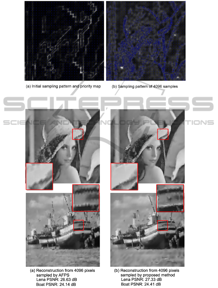
Figure 5: Example of sampling patterns of lena, and the corresponding priority maps. Blue dots are sampled pixel locations
and brighter spots correspond to higher priorities.
Figure 6: Result comparison with AFPS (Devir and Lindenbaum, 2007), at 4096 samples.
Kernel-basedAdaptiveImageSampling
31

both sampling methods, the proposed method en-
hances the visual quality of the reconstructed image
by focusing on sampling in structured regions such as
edges. Therefore, the consequent image reconstructed
from the basic linear bivariate splines has a similar
sharpening effect as images enhanced by kernel re-
gression (Takeda et al., 2007).
More experimental results are provided in Table.1,
showing the ability of the proposed method to capture
the embedded image structure at early stage of sam-
pling.
Table 1: Performance comparison in PSNR (dB).
Target Method 0.2 b/p 0.3 b/p 0.5 b/p
Lena AFPS 23.63 24.83 26.63
KbAS 23.72 25.32 27.33
Barbara AFPS 22.36 23.69 25.09
KbAS 22.44 23.98 25.37
Boat AFPS 21.62 22.62 24.14
KbAS 21.95 22.91 24.41
Cameraman AFPS 21.62 23.21 25.46
KbAS 21.98 23.59 25.75
Peppers AFPS 22.16 23.41 25.54
KbAS 22.58 24.17 25.98
5 CONCLUSIONS
In this paper, we proposed the Kernel-based Adap-
tive Sampling method that is able to progressively
sample/reconstruct an image, without the need of
pre-processing or compression of the image. The
proposed method makes use of the prior knowledge
about natural images embedded in the framework of
kernel construction, and is able to identify at early
stages pixel locations that are more significant to im-
prove the reconstruction quality of the image. Recon-
structed images from samples retrieved from the pro-
posed method have higher image quality measured in
PSNR, as well as better visual quality by virtue of the
steerable kernel modeling.
REFERENCES
Chang, C.-C., Li, Y.-C., and Lin, C.-H. (2008). A
novel method for progressive image transmission us-
ing blocked wavelets. AEU-International Journal of
Electronics and Communications, 62(2):159–162.
Chang, C.-C. and Lu, T.-C. (2006). A wavelet-based pro-
gressive digital image transmission scheme. In In-
novative Computing, Information and Control, 2006.
ICICIC’06. First International Conference on, vol-
ume 2, pages 681–684. IEEE.
Chang, C.-C., Shiue, F.-C., and Chen, T.-S. (1999).
A new scheme of progressive image transmission
based on bit-plane method. In Communications,
1999. APCC/OECC’99. Fifth Asia-Pacific Conference
on... and Fourth Optoelectronics and Communica-
tions Conference, volume 2, pages 892–895. IEEE.
Chen, T. and Chang, C. (1997). Progressive image transmis-
sion using side match method. Information Systems
and Technologies for Network Society, pages 191–
198.
Demaret, L., Dyn, N., and Iske, A. (2006). Image com-
pression by linear splines over adaptive triangulations.
Signal Processing, 86(7):1604–1616.
Devir, Z. and Lindenbaum, M. (2007). Adaptive range sam-
pling using a stochastic model. Journal of computing
and information science in engineering, 7(1):20–25.
Eldar, Y., Lindenbaum, M., Porat, M., and Zeevi, Y. (1997).
The farthest point strategy for progressive image sam-
pling. Image Processing, IEEE Transactions on,
6(9):1305–1315.
Jiang, J., Chang, C., and Chen, T. (1997). Selective progres-
sive image transmission using diagonal sampling tech-
nique. In Proceedings of International Symposium on
Digital Media Information Base, pages 59–67.
Rajesh, S., Sandeep, K., and Mittal, R. (2007). A fast
progressive image sampling using lifting scheme and
non-uniform b-splines. In Industrial Electronics,
2007. ISIE 2007. IEEE International Symposium on,
pages 1645–1650. IEEE.
Said, A. and Pearlman, W. A. (1996). A new, fast, and
efficient image codec based on set partitioning in hi-
erarchical trees. Circuits and systems for video tech-
nology, IEEE Transactions on, 6(3):243–250.
Shapiro, J. M. (1993). Embedded image coding using ze-
rotrees of wavelet coefficients. Signal Processing,
IEEE Transactions on, 41(12):3445–3462.
Skodras, A., Christopoulos, C., and Ebrahimi, T. (2001).
The jpeg 2000 still image compression standard. Sig-
nal Processing Magazine, IEEE, 18(5):36–58.
Takeda, H., Farsiu, S., and Milanfar, P. (2007). Kernel
regression for image processing and reconstruction.
Image Processing, IEEE Transactions on, 16(2):349–
366.
Tzou, K.-H. (1986). Progressive image transmission: a re-
view and comparison of techniques. Optical Engi-
neering, 26(7):267581–267581.
Verma, R., Verma, R., Sree, P. S. J., Kumar, P., Sidda-
vatam, R., and Ghrera, S. (2010). A fast progres-
sive image transmission algorithm using linear bivari-
ate splines. In Contemporary Computing, pages 568–
578. Springer.
VISAPP2014-InternationalConferenceonComputerVisionTheoryandApplications
32
