Chemical Master Equations

A Mathematical Scheme for the Multi-site Phosphorylation Case

∗

Alessandro Borri, Francesco Carravetta, Gabriella Mavelli and Pasquale Palumbo

Istituto di Analisi dei Sistemi ed Informatica “A. Ruberti”, Consiglio Nazionale delle Ricerche (IASI-CNR),

Viale Manzoni 30, 00185 Roma, Italy

Keywords:

Systems Biology, Chemical Master Equation, Markov Processes, Enzymatic Reactions.

Abstract:

The Chemical Master Equation (CME) provides a fruitful approach for the stochastic description of complex

biochemical processes, because it is able to cope with random ﬂuctuations of the chemical agents and to ﬁt

the experimental behavior in a more accurate way than deterministic concentration equations. In this work,

our attention is focused on modeling and simulation of multisite phosphorylation/dephosphorylation cycles,

by using the quasi-steady state approximation of enzymatic kinetics. The CME dynamics is written from the

coefﬁcients of the deterministic reaction-rate equations and the stationary distribution is computed explicitly,

according to a recently developed realization scheme. Simulations are included to provide a comparison with

Monte Carlo methods in terms of computational complexity.

1 INTRODUCTION

Understanding complex cellular processes is a major

challenge facing present-day biology. Systems Bi-

ology is an approach that tackles the study of such

complex systems and is characterized by the fact that

molecular analysis - often at the genomic scale - is in-

tegrated with modeling, parameter identiﬁcation, sim-

ulation analysis and control theory. Within this ap-

proach, biological processes are taken to be the re-

sults of complex, coordinated, dynamic, nonlinear in-

teractions of a large number of components, which

are affected by time and space constraints. The de-

velopment of efforts in the Systems Biology research

ﬁeld will allow to elucidate relevant central features

of the more basic complex cellular functions (such

as cycle, growth, and so on) as well as to identify

their system-level properties, ultimately contributing

to shed more light on diseases arising as the impair-

ment metabolic functions such as cancer, diabetes,

etc. To this aim, a successful analysis of the com-

plex mechanisms arising in System Biology requires

the application of more and more efﬁcient methods

for modeling such complex cellular systems.

As far as the networks of biochemical reactions,

there is an increasing interest in the development and

analysis of stochastic models, due to the preminent

∗

This work is partially supported by project IN-

TEROMICS.

role of ﬂuctuations whenever a low number of

molecules is involved, (Mettetal and van Oudenaar-

den, 2007). Indeed, in a single cell environment, the

concentration of molecules can be low, so molecular

species can be found with a number of copies ranging

from hundreds to thousands. The small number of

molecules involved and the inherent stochasticity

of biochemical processes justify the necessity of

the stochastic approach to cope with intracellular

processes, (Van Kampen, 2007).

The biochemical complex machinery is largely

based on enzymatic reactions. Among the covalent

enzymatic-catalyzed modiﬁcations of substrates,

phosphorylation and dephosphorylation reactions

catalyzed by kinases and phosphatases, respectively,

provide a reversible post-translational substrate

modiﬁcation that is central to cellular signalling

and regulation. In (Qu et al., 2003) it has been

proposed that multisite phosphorylation of tar-

get proteins by cyclin-dependent kinase proteins

is the likely source of nonlinear kinetic effects

in cell cycle control mechanisms. In particular,

dual phosphorylation/dephosphorylation cycles are

widely diffused within cellular systems and are

crucial for the control of complex responses such as

learning, memory, and cellular fate determination.

The majority of studies on biophysical analysis of

phosphorylation/dephosphorylation cycle have been

performed in an averaged, deterministic framework

681

Borri A., Carravetta F., Mavelli G. and Palumbo P..

Chemical Master Equations - A Mathematical Scheme for the Multi-site Phosphorylation Case.

DOI: 10.5220/0004632306810688

In Proceedings of the 3rd International Conference on Simulation and Modeling Methodologies, Technologies and Applications (BIOMED-2013), pages

681-688

ISBN: 978-989-8565-69-3

 2013 SCITEPRESS (Science and Technology Publications, Lda.)

based on the Michaelis-Menten approach (Michaelis

and Menten, 1913). As stated above about generic

molecules, indeed in a single cell the substrate

and enzyme concentration can be low, being thus

necessary to study these cases within a stochastic

framework. Examples of biochemical reactions with

low number of substrates and involved enzymes

present at low concentrations are the phosphoryla-

tion/dephosphorylation cycle of AMPA-Receptors

(AMPARs) in a single synaptic spine and have been

treated in (Castellani et al., 2001; Whitlock et al.,

2006). In (Castellani et al., 2001) it has been pro-

posed a synaptic receptors model (AMPAR model)

which, at a molecular-microscopic level, is a candi-

date for memory storage and switching behavior, and

a kinetic scheme of the enzymatic reactions describ-

ing the AMPAR double phosphorylation channel has

been given. It has been stressed that the AMPAR

modiﬁcation, a 2-step phospho/dephosphorylation

cycle, guaranties the synaptic plasticity and exhibits

bistability for a wide range of parameters, consistent

with values derived from biological literature.

In this paper we investigate the Chemical

Master Equation (CME) approach applied to

model in a stochastic framework the phosphoryla-

tion/dephosphorylation cycle. Indeed, the CMEs

provides an appropriate description of complex cellu-

lar processes, (Van Kampen, 2007; Gillespie, 1977).

It is a powerful method even with signiﬁcant sim-

pliﬁcations, such as spatial homogeneity of volumes

where the chemical reactions under investigation are

taking place. The CME is a promising approach for

Systems Biology modelling for a variety of reasons,

such as its capability of coping with ﬂuctuations and

chemical ﬂuxes and of well ﬁtting experimental data

in the today widespread single cell experiments, and

its capability to capture and explain the deviation

from Gaussianity observed in various gene expression

experiments (such as stress or metabolic response,

growth of the nuclear protein amount observed in

senescent cells, and so on). It results more infor-

mative of the real behavior of the system than the

deterministic approach, since the results obtained in

a deterministic framework cannot describe diffusion

effects due to ﬂuctuations and chemical currents

capable to drive switching from one equilibrium to

the other. Such mechanism has a relevant role also

in neuronal plasticity phenomena, (Castellani et al.,

2009). In (Bazzani et al., 2012) the stationary dis-

tribution provided by the two-dimensional chemical

master equation for a well-known model of a two

step phosphorylation/dephosphorylation cycle has

been studied, by using the quasi-steady state approx-

imation of enzymatic kinetics. Authors pointed out

the possibility for the molecule distribution shape to

be controlled (in particular changed from a unimodal

distribution to a bimodal distribution) by chemical

ﬂuxes occurring in the biochemical system under

investigation. This phenomenon corresponds to the

typical mechanism that is adopted by such system

to obtain a plastic behavior, for example when any

kind of exogenous chemical messenger is present, by

changing the properties of the biochemical reaction

occurring inside the cell.

The paper is organized as follows: in Section 2 we

review some structural properties of the Master Equa-

tion and address the efﬁcient computation of its equi-

librium solution. In Section 3, we illustrate the case

study of multiple phosphorylation for an arbitrary

number of sites. In Section 4 we propose some sim-

ulation results concerning the case of a triple phos-

phorylation framework. Section 5 offers concluding

remarks.

2 THE CHEMICAL MASTER

EQUATION

Consider M (bio)chemical species Y

,...,Y

involved

in q chemical reactions (Ullah and Wolkenhauer,

2011) described by the stoichiometric coefﬁcients β

for any species j = 1,...,M and for any reaction i =

1,...,q. The Chemical Master Equation (CME) de-

scribes the time evolution of the probability of being

in one of the N ≤ +∞ possible conﬁgurations (states)

at any time (Van Kampen, 2007). More generally, the

CME is the dynamic equation of a continuous-time

discrete-state stochastic Markov process. If N is ﬁ-

nite, the equations for the joint probabilities can be

collected in the form of an autonomous positive lin-

ear system (Farina and Rinaldi, 2000):

P = GP , P ∈ R

, (1)

where G is called inﬁnitesimal generator of the

Markov process.

We deﬁne as n(t) = (n

(t),... , n

(t)) the state of

the system at time t, with i-th component n

(t) ∈ N

denoting the number of copies of species Y

at time

t. The generic element G

of G is the propensity

,...,α

,...,n

of reaching the state v

= (n

+ α

,...,n

) from the state v

= (n

,...,n

Depending on whether or not the system of re-

actions is closed (the total mass is conserved) and

according to the number of distinct elements form-

ing the M species, the values of some components of

the vector state n(t) can be inferred from the others,

which makes the state representation redundant. We

SIMULTECH2013-3rdInternationalConferenceonSimulationandModelingMethodologies,Technologiesand

Applications

682

will henceforth assume that the M species are inde-

pendent, i.e. the state representation is minimal (non-

redundant). The interested reader is referred to (Borri

et al., 2013) for a deeper discussion on these and on

the following concepts.

Note that different ways of aggregation of the

probabilities in the vector P may produce different

properties of the linear system in (1). In particular,

one can consider the following recursive partitioning:

,...,n

M−1







,...,n

M−1

,...,n

M−1

,...,n

M−1







∈ R

, (2)

with 0 ≤ n

≤ N

, with N

being the maximum number

of allowed copies of species Y

, and p

,...,n

being

the joint probability of having n

copies of species Y

for all i = 1,...,M. Then, the following vectors of

probabilities can be recursively deﬁned

,...,n







,...,n

i+1







∈ R

i+1

+1)×···×(N

+1)

(3)

for 1≤ i≤ M−2. This leads to the deﬁnition of vector

P , entailing all the joint probabilities involved by the

CME:













∈ R

+1)×···×(N

+1)

. (4)

The way of collecting the probabilities in P as in

(2)–(4) induces a recursive block partitioning on ma-

trix G, according to (1). In case the stoichiometric

coefﬁcients satisfy the unitary step property:

∈ {−1,0, 1},i ∈ {1,...,q}, j ∈ {1,...,M}, (5)

an interesting recursivestructure of the CME dynamic

equations can be pointed out:

Proposition 1. Consider a continuous-time Markov

process describing a set of q chemical reactions in-

volving M independent (bio)chemical species and de-

scribed by a set of stoichiometric coefﬁcients {β

}

satisfying (5). Then the inﬁnitesimal generator G

has the following block-tridiagonal structure (see e.g.

(Carravetta, 2011)):

G=Φ



},{G

−1

};n









−1

0 ··· ···

−1

0 ···

−2

−1

0 ··· · · ·

0 G

−1







(6)

where the

0 entries are zero matrices of proper dimen-

sions. Furthermore, all the non-zero blocks of G are

block-tridiagonal with the same structure of G.

The operator Φ

({A

},{B

},{C

};i) used in (6) is

called block-tridiagonal matrix builder and is deﬁned

as follows

({A

},{B

},{C

};i) :=







0 ···

ν−2

ν−1

0 ···

0 A

ν−1







(7)

where {A

}, {B

}, {C

} are sequences of suitably

dimensioned square matrices, and the

0 entries are

zero matrices of proper dimensions. A network of

chemical reactions satisfying (5) allows simultane-

ous changes of unitary amount in the state variables

and is later referred as generalized one-step process

or unitary process. It is possible to show that (5) is

the mildest condition preserving the recursive block-

tridiagonal structure of G.

The main consequenceof Proposition 1 is that G is

sparse, which reveals to be useful to carry out classi-

cal tasks as the computation of the stationary solution

of the CME, satisfying

GP = 0. (8)

The following result, based on an interpretation of

the biochemical network in terms of Algebraic Graph

Theory (Bullo et al., 2009), characterizes the prop-

erty of uniqueness of the CME stationary distribution,

which makes the study of the equilibrium problem (8)

independent of the initial state.

Proposition 2. The stationary distribution P

of a

continuous-time Markov process is unique if and only

if the digraph associated with the Markov process has

a globally reachable vertex. Under this assumption, 0

is a simple eigenvalue of G with right eigenvector u

and the stationary distribution is given by P

ChemicalMasterEquations-AMathematicalSchemefortheMulti-sitePhosphorylationCase

683

As an alternative approach to the computation of

in terms of the right eigenvector u

of G, Propo-

sitions 1 and 2 allow an efﬁcient computation of the

solution of (8) by means of Gaussian elimination:

Proposition 3. The algorithm of Gaussian elimi-

nation to solve the stationary equation GP = 0 in

unitary-step processes is performed in time O (N

where N is the number of rows of G.

Note that the complexity of the Gaussian Elimina-

tion for dense matrices is O(N

3 MULTI-SITE

PHOSPHORYLATION

This section is devoted to formalizing, in the CME

mathematical setting, the multi-site phosphorylation

reaction framework.

3.1 Writing the Reaction-rate

Equations

Consider the case of only M = 2 phosphorylationsites

(see e.g. (Bazzani et al., 2012)), depicted in Fig. 1,

involvingM+1= 3 species and 2 enzymes (kinase E

and phosphatase E

). Such a framework is formalized

by the following set of q = 2M = 4 reactions:











(0)

−→ A

(1)

−→ A

(2)

(1)

−→ A

(0)

(2)

−→ A

(1)

where the species A

(0)

, A

(1)

, A

(2)

are the

non-phosphorylated, phosphorylated and double-

phosphorylated substrate, respectively. If one con-

siders the double-site phosphorylation as a closed

system (the total substrate concentration is constant

(0)

]+ [A

(1)

]+ [A

(2)

] = A

tot

), the number of indepen-

dent species is M = 2.

We now address the general M-site phosphoryla-

tion case, illustrated in Fig. 2. We can consider the

case of closed system, so that the species A

(i)

may be

intended to be the i-times phosphorylated substrate,

for i = 0,...,M, and the total substrate concentration

is constant

∑

i=0

(i)

] = A

tot

. The odd-indexed reac-

tions are catalyzed by the kinase E

(i−1)

] + [E

]

2i−1

↼−−−

−−−⇁

2i−1

OFF

(i−1)

]

2i−1

−−−→ [A

(i)

] + [E

]

(9)

with i = 1, ..., M, while the even-indexed reactions

are activated by the phosphatase E

(i)

] + [E

]

↼−−−

−−−⇁

OFF

(i)

]

−→ [A

(i−1)

] + [E

] (10)

with i = 1,...,M, for a total number of reactions

equal to q = 2M.

The left-hand M pairs of reactions in (9)–(10) are

considered at the equilibrium (quasi-steady-state hy-

pothesis), thus the corresponding 2M deterministic

Michaelis-Menten (MM) equations rewrite:

d[A

(i−1)

]

2i−1

(i−1)

][E

]−K

2i−1

OFF

(i−1)

]=0

d[A

(i)

]

(i)

][E

]−K

OFF

(i)

]=0

for i = 1,...,M. Hence, by setting the dissociation

coefﬁcients k

:= K

OFF

, j = 1,...,2M, one gets

the equilibrium conditions:







(i−1)

]

(i−1)

][E

]

2i−1

(i)

]

(i)

][E

]

for i = 1,...,M. We now focus on the right-hand

reactions in (9)–(10), where we replace the terms

] with their equilibrium values [A

]

, for j =

1,...,2M and k = 1,2. One gets:

(i−1)

][E

]

2i−1

−−−→ [A

(i)

] + [E

], (11)

(i)

][E

]

−→ [A

(i−1)

] + [E

]. (12)

Note that the generic species A

(i)

, for i = 1,...,M, ap-

pears in 4 distinct reactions:

(i−1)

][E

]

2i−1

−−−→ [A

(i)

] + [E

(i)

][E

]

−→ [A

(i−1)

] + [E

(i)

][E

]

2i+1

−−−→ [A

(i+1)

] + [E

(i+1)

][E

]

2(i+1)

−−−→ [A

(i)

] + [E

which lead to the following MM equation, for any i:

d[A

(i)

]

2i−1

][A

(i−1)

] −

][A

(i)

]

−

2i+1

][A

(i)

] +

2(i+1)

][A

(i+1)

]. (13)

SIMULTECH2013-3rdInternationalConferenceonSimulationandModelingMethodologies,Technologiesand

Applications

684

(0)

(1)

(2)

Figure 1: Double-site Phosphorylation.

2 4

2i − 1

2i + 1

2(i + 1)

(0)

(1)

(i)

(M −1)

(M )

2M − 1

2M − 3

2M − 2

Figure 2: Multi-site Phosphorylation.

Note that i = 0, i = M are special cases because some

terms are neglected:

d[A

(0)

]

= −

][A

(0)

] +

][A

(1)

], (14)

d[A

(M)

]

2M−1

][A

(M−1)

] −

][A

(M)

(15)

The following mass-balance constraints on the total

substrate concentration and on the enzymes:











∑

i=0

(i)

] = A

tot

] +

∑

i=1

(i−1)

]

2i−1

] = E

1,tot

] +

∑

i=1

(i)

]

] = E

2,tot

(16)

lead to the a minimal representation of the process by

means of M independent species. For instance, we

choose x

= [A

(i)

] for i = 1,...,M and, from (13), we

are able to describe the system in terms of M coupled

differential equations, called reaction-rate equations:











˙x

(x)x

−



(x) +

(x)



(x)x

˙x

2i−1

(x)x

i−1

−



(x) +

2i+1

(x)



2(i+1)

(x)x

i+1

˙x

2M−1

(x)x

M− 1

−

(x)x

(17)

where x

:= [A

(0)

] and E

(x), E

(x) are given by:











= 1 −

∑

i=1

(x) =

1,tot

∑

i=1

i−1

2i−1

(x) =

2,tot

∑

i=1

(18)

3.2 From the Reaction-rate Equations

to the Master Equation

In (17)–(18), we built a minimal deterministic repre-

sentation of the M-site phosphorylation by means of

a system of M ordinary differential equations (ODEs)

with respect to the M variables x

,...,x

, where x

represents the normalized concentration of species

, i.e. of the i-times phosphorylated substrate. It

is deeply discussed in the related literature how the

reaction-rate approach fails to capture the inherent

randomness of biochemical phenomena, especially in

the presence of a low number of molecules (Van Kam-

pen, 2007). In the following, we build a stochas-

tic representation of the chemical process in terms of

Master Equations.

A common approach to infer the CMEs from the

ODEs consists in turning the real-valued concentra-

tion variables x

into the integer values n

, represent-

ing the copies of species Y

, according to the mass-

balance constraint:

= n

TOT

−

∑

i=1

As a ﬁrst step, we need to write the stoichiometric

coefﬁcients for each reaction.

Odd-indexed Reactions. The generic reaction

2i − 1, for i = 1,...,M, “generates” a molecule of

species Y

and “annihilates” a molecule of species

i−1

, from (11). Hence the vector of stoichiometric

ChemicalMasterEquations-AMathematicalSchemefortheMulti-sitePhosphorylationCase

685

coefﬁcients

2i−1

= (β

2i−1,1

,...,β

2i−1,M

) for these re-

actions is given by:

2i−1, j











1 j = i,

−1 j = i− 1,

0 otherwise.

(19)

Even-indexed Reactions. The generic reaction 2i,

for i = 1,...,M, reverses the reaction 2i− 1, namely it

generates a molecule of species Y

i−1

and annihilates

one of species Y

, from (12). Hence the vector of stoi-

chiometric coefﬁcients

= (β

2i,1

,...,β

2i,M

) for these

reactions is given by:

2i, j











−1 j = i,

1 j = i− 1,

0 otherwise.

(20)

Writing the Matrix G. We are now ready to

write the CME by computing the generic element g

(propensity), with the shortcuts n = (n

,...,n

) and

α = (α

,...,α

). By comparison with the equation of

species i in (17):

˙x

2i−1

(x)x

i−1

−



(x) +

2i+1

(x)



2(i+1)

(x)x

i+1

(21)

and taking into account the deﬁnition of the vectors of

stoichiometric coefﬁcients in (19)–(20), one can de-

ﬁne:











2i−1

(n)n

i−1

α =

2i−1

,i = 1,...,M,

2(i+1)

(n)n

i+1

α =

2(i+1)

,i = 1,...,M,

−

∑

i=1



(n)+

2i+1

(n)



α = 0,

0 otherwise,

(22)

where 0 = (0,...,0). Intuitively, the deﬁnition in (22)

is obtained from (21) by regarding the positive ad-

dends as generation terms (i.e. creating a molecule)

and the negativeones as recombination terms (i.e. an-

nihilating a molecule) of the associated biochemical

reactions. The dynamic matrix G of the CME can be

written as in (6), where the scalar blocks are deﬁned

from the propensities as:

,...,α

,...,n







,...,α

,...,n

if (α

,...,α

) 6= 0,

−

∑

,...,

,...,n

otherwise,

(23)

and the general blocks are recursively deﬁned in

terms of the matrix builder in (7) as:

,...,α

,...,n

=Φ

i+1



,...,α

,...,n

i+1

,...,α

,...,n

i+1

},{G

,...,α

,−1

,...,n

i+1

};n

i+1



(24)

for 1≤ i ≤ M−1, 0 ≤ n

≤ N

TOT

, 0 ≤ |α

| ≤ N

TOT

It can be shown (see e.g. (Van Kampen, 2007))

that the deterministic reaction-rate approach is a ﬁrst-

order approximation of the dynamics of the mean

value of the CME.

4 SIMULATION RESULTS

In the following, we restrict our attention to the case

M = 3 (triple phosphorylation) and we compare the

performance between computing the stationary distri-

bution explicitly, based on the results in Section 2, and

obtaining it by means of statistical methods, in par-

ticular the Gillespie Stochastic Simulation Algorithm

(SSA) (Gillespie, 1977).

For M = 3, we have q = 6 reactions. We assume

TOT

= 40 and E

1,TOT

= E

2,TOT

= 1. The dimen-

sion of G is N = 41

> 64, 000, but an inspection

of the associated states reveals that a large subset of

those are not reachable (in the sense of Munsky et al.

(Munsky and Khammash, 2008)) because they vio-

late the mass-balance constraints, hence they have a

zero steady-state probability. If one erases a priori

the components referred to those states from the mas-

ter equation, a reduced matrix

G is obtained, whose

kernel is 1-dimensional. This ensures the uniqueness

of the stationary distribution

, deﬁned over the set

of reachable states of the Markov Process. In this par-

ticular case, just

N = 12, 341 conﬁgurations are ad-

missible states.

The values of the chosen parameters are: k

= 1, k

= k

= 1.8, k

= k

= 2.2, v

= v

= 1,

= v

= 1.1, v

= v

= 1.2. We apply the formaliza-

tion in Section 3 and perform numerical simulations

in the Matlab suite on an Apple MacBook Pro laptop

with 2.5 GHz Intel Core i5 CPU and 16 GB RAM.

We started with the stochastic simulation. We

considered as initial state n(0) = (0, 0,0), meaning

that n

= n

TOT

, i.e. all the molecules are non-

phoshorylated at the beginning. We performed 10

Monte Carlo runs of SSA, with a time horizon of

500 seconds. The average number of reactions for

each SSA run was 9925. The whole computation took

more than 12 hours.

We then compared 3 methods of computing the

theoretical stationary distribution:

(1) We computed the eigenvalues and eigenvectors of

matrix

G by means of Matlab’s eig routine. Ac-

SIMULTECH2013-3rdInternationalConferenceonSimulationandModelingMethodologies,Technologiesand

Applications

686

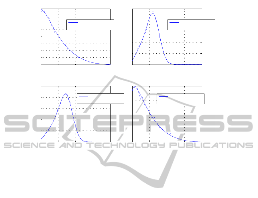
0 10 20 30 40

0.01

0.02

0.03

0.04

0.05

0.06

0.07

0.08

Stationary Distribution, Species A

(0)

Theoretical Distribution

Statistical Distribution

0 10 20 30 40

0.02

0.04

0.06

0.08

0.1

Stationary Distribution, Species A

(1)

Theoretical Distribution

Statistical Distribution

0 10 20 30 40

0.02

0.04

0.06

0.08

0.1

Stationary Distribution, Species A

(2)

Theoretical Distribution

Statistical Distribution

0 10 20 30 40

0.01

0.02

0.03

0.04

0.05

0.06

0.07

0.08

Stationary Distribution, Species A

(3)

Theoretical Distribution

Statistical Distribution

Figure 3: Steady-state marginal distributions. The solid line is the theoretical distribution computed explicitly according to

the methods illustrated in the paper. The dashed line is the statistical distribution provided by 5,000 Monte Carlo runs of the

Gillespie Algorithm.

cording to Proposition 2, the stationary distribu-

tion is the right eigenvector corresponding to the

zero eigenvalue of

G. The procedure took 2785

seconds.

(2) According to Proposition 3, we computed

means of an ad hoc implementation of the Gaus-

sian Elimination method to compute the solution

P = 0. Although it is very accurate, this

method was outperformed (in terms of time com-

plexity) by method (1) and the elapsed time is

comparable to the Gillespie method.

(3) We computed the matrix exponential e

, by

means of the Matlab routine expm, and we con-

sidered as initial condition

P (0) the probability

vector with value equal to 1 for the component re-

ferred to the state n(0) and 0 elsewhere. We then

computed the steady-state distribution by means

of a ﬁxed-point iteration for the recursion p

k+1

, initialized with p

P (0), which is the ex-

act discretization of the CME with unitary sam-

pling time, and where we used the stopping con-

dition kp

k+1

− p

k ≤ 10

−6

. Most of the time in

this case is spent in computing the matrix expo-

nential, computed in 357 seconds. The ﬁxed point

iteration took 88 seconds to reach the steady state.

The methods above return the same distribution,

with a relative difference lower than 10

−6

(in norm).

The plots in Fig. 3 show the agreement between the

statistical estimation of the steady-state solution and

the theoretical stationary distribution. Due to the sav-

ing in terms of computational resources, the explicit

computation is preferable.

5 CONCLUSIONS

In this work we illustrated the application of some re-

sults about the efﬁcient computation of the stationary

distribution of the Chemical Master Equation in the

biochemical framework of multisite phosphorylation.

Based on a recently developed representation scheme,

it is shown how the proposed approach results to be

accurate and with limited computational burden, es-

pecially with respect to the extensive use of statistical

Monte Carlo methods.

REFERENCES

Bazzani, A., Castellani, G. C., Giampieri, E., Remondini,

D., and Cooper, L. N. (2012). Bistability in the chem-

ical master equation for dual phosphorylation cycles.

The Journal of Chemical Physics, 136(23):235102.

Borri, A., Carravetta, F., Mavelli, G., and Palumbo, P.

(2013). Some results on the structural properties and

ChemicalMasterEquations-AMathematicalSchemefortheMulti-sitePhosphorylationCase

687

the solution of the chemical master equation. In Pro-

ceedings of the 2013 American Control Conference

(ACC 2013), Washington, DC, USA.

Bullo, F., Cortes, J., and Martinez, S. (2009). Distributed

Control of Robotic Networks. Applied Mathematics

Series. Princeton.

Carravetta, F. (2011). 2-d-recursive modelling of homoge-

neous discrete gaussian markov ﬁelds. IEEE Transac-

tions on Automatic Control, 56(5):1198–1203.

Castellani, G. C., Bazzani, A., and Cooper, L. N. (2009).

Toward a microscopic model of bidirectional synaptic

plasticity. Proceedings of the National Academy of

Sciences, 106(33):14091–14095.

Castellani, G. C., Quinlan, E. M., Cooper, L. N., and Shou-

val, H. Z. (2001). A biophysical model of bidirectional

synaptic plasticity: Dependence on ampa and nmda

receptors. Proceedings of the National Academy of

Sciences, 98(22):12772–12777.

Farina, L. and Rinaldi, S. (2000). Positive Linear Systems:

Theory and Applications. Pure and Applied Mathe-

matics Series. John Wiley & Sons, Inc.

Gillespie, D. T. (1977). Exact stochastic simulation of

coupled chemical reactions. The Journal of Physical

Chemistry, 81(25):2340–2361.

Mettetal, J. T. and van Oudenaarden, A. (2007). Necessary

noise. Science, 317(5837):463–464.

Michaelis, L. and Menten, M. (1913). Kinetics of invertase

action. Biochem. Z, 49:333–369.

Munsky, B. and Khammash, M. (2008). The ﬁnite state pro-

jection approach for the analysis of stochastic noise in

gene networks. IEEE Transactions on Automatic Con-

trol, 53(Special Issue on Systems Biology):201–214.

Qu, Z., Weiss, J. N., and MacLellan, W. R. (2003). Reg-

ulation of the mammalian cell cycle: a model of the

g1-to-s transition. American Journal of Physiology -

Cell Physiology, 284(2):C349–C364.

Ullah, M. and Wolkenhauer, O. (2011). Stochastic Ap-

proaches for Systems Biology. Springer.

Van Kampen, N. G. (2007). Stochastic Processes in Physics

and Chemistry, Third Edition. North Holland.

Whitlock, J. R., Heynen, A. J., Shuler, M. G., and Bear,

M. F. (2006). Learning induces long-term potentia-

tion in the hippocampus. Science (New York, N.Y.),

313(5790):1093–1097.

SIMULTECH2013-3rdInternationalConferenceonSimulationandModelingMethodologies,Technologiesand

Applications

688