
Prediction based – High Frequency Trading on Financial Time Series
Farhad Kia and Janos Levendovszky
Department of Telecommunications, Budapest University of Technology and Economics,
Magyar Tudósok krt. 2., Budapest, Hungary
Keywords: Feedforward Neural Networks, High Frequency Trading, Financial Time Series Prediction.
Abstract: In this paper we investigate prediction based trading on financial time series assuming general AR(J)
models and mean reverting portfolios. A suitable nonlinear estimator is used for predicting the future values
of a financial time series will be provided by a properly trained FeedForward Neural Network (FFNN)
which can capture the characteristics of the conditional expected value. In this way, one can implement a
simple trading strategy based on the predicted future value of an asset price or a portfolio and comparing it
to the current value. The method is tested on FOREX data series and achieved a considerable profit on the
mid price. In the presence of the bid-ask spread, the gain is smaller but it still ranges in the interval 2-6
percent in 6 months without using any leverage. FFNNs were also used to predict future values of mean
reverting portfolios after identifying them as Ornstein-Uhlenbeck processes. In this way, one can provide
fast predictions which can give rise to high frequency trading on intraday data series.
1 INTRODUCTION
In the advent high speed computation and ever
increasing computational power, algorithmic trading
has been receiving a considerable interest (A Hanif,
2012) (Pole, 2007) (Kissell, 2006) (Peter Bergan,
2005). The main focus of research is to develop real-
time algorithms which can cope with portfolio
optimization and price estimation within a very
small time interval enabling high frequency, intraday
trading. In this way, fast identification of favorable
patterns on time series becomes feasible on small
time scales which can give rise to profitable trading
where asset prices follow each other in sec or msec
range.
Several papers have been dealt with algorithmic
trading by using fast prediction algorithms (Naik et
al., 2012); (Y. Zuo, 2012) or by identifying mean
reverting portfolios (J.W., 2002) (D’Aspremont,
2011) (Balvers et al., 2000). The paper (L., 2012)
uses linear prediction which however proves to be
poor to capture the complexity of the underlying
time series. Other methods (D’Aspremont, 2011);
(Balvers et al., 2000) are focused on identifying
mean reverting portfolios and launch a trading action
(e.g. buy) if the portfolio is out of the mean and
taking the opposite action when it returns to the
mean.
In our approach, we focus on prediction based
trading by estimating the future price of the time
series by using a nonlinear predictor in order to
capture the underlying structure of the time series.
The investigated time series can either refer to
foreign exchange rates, single asset prices or the
value of a previously optimized portfolio. By using
FFNNs, which exhibit universal representation
capabilities, one can model the nonlinear AR(J)
process (the current value of the time series depends
on J previous values and corrupted by additive
Gaussian noise). Assuming the price series to be a
nonlinear AR(J) process, we first develop the
optimal trading strategy and then approximate the
parameters of nonlinear AR(J) by an FFNN.
In this way, one can obtain a fast adaptive
trading procedure which, in the first stage, runs a
learning algorithm for parameter optimization based
on some observed prices and then, in the second
stage, provides near optimal estimation of future
prices. The numerical results obtained on Forex rates
have demonstrated that the method is profitable and
achieves more than 1% profit in one month with
leverage 1:1 which can be much bigger if we use
leverage.
The paper treats this material in the following
structure:
In section 2, the model is outlined;
In section 3 the optimal strategy is derived first for
trading on mid-prices and then it is extended to
502
Kia F. and Levendovszky J..
Prediction based – High Frequency Trading on Financial Time Series.
DOI: 10.5220/0004555005020506
In Proceedings of the 5th International Joint Conference on Computational Intelligence (NCTA-2013), pages 502-506
ISBN: 978-989-8565-77-8
Copyright
c
2013 SCITEPRESS (Science and Technology Publications, Lda.)

trading in the presence of bid-ask spread;
In section 4 numerical results and performance
analysis is given;
In section 5 some conclusions are drawn.
2 THE MODEL
Let us assume that we trade on the mid prices, the
corresponding asset price time series is denoted by
n
x
and follows a nonlinear AR(J) process
1,...,nnnJn
xFx x
(2.1)
where F is a Borel measurable function and
0,
n
N
i.i.d.r.v.-s, being independent of
n
x
.
For trading, we construct an estimator
11
,..., , ,..., ,
nnnJM
xNetx xw w Net
xw
,
(2.2)
where
() ( 1) (1)
, ... ...
LL
niijnmnm
ij m
xNet w w wx
xw
is a Feedforward neural Network (FFNN) depicted
by Figure 2.1 and vector w denotes the free
parameters subject to training.
Figure 2.1: The structure of feed forward neural network
(FFNN).
Trading is performed as follows:
Stage 1. Observing a historical time series and
forming a training set
() ()
, , 1,...,
nn
n
x
nN
x
where
()
1
,...,
n
nJ n
x
x
x
.
Stage 2. Training the weights by minimizing the
objective function
2
()
1
min ,
n
n
xNet
N
w
xw
by the
back propagation (BP) algorithm.
Stage 3. Trading on the real data as follows:
Calculate
()
,
n
n
xNet xw
,where
()
1
,...,
n
nJ n
x
x
x
and we are in time instant
1n
.
If
1nn
x
x
then buy at time instant
1n
and sell at
time instant
n
. (2.3)
If
1nn
x
x
then sell at time instant
1n
and buy at
time instant
n
. (2.4)
It can be easily proven that this is the optimal
strategy, as far as the expected profit maximization
is concerned.
3 PORTFOLIO OPTIMIZATION
BY MEAN REVERSION
We view the asset prices as a first order, vector
autoregressive VAR (1) process. Let
,it
s
denote the
price of asset
i at time instant t, where
1,...,in
and
1,...,tm
are positive integers and assume that
1, ,
( ,..., )
T
ttnt
s
ss
is subject to a first order vector
autoregressive process, VAR (1), defined as follows:
1
,
tt t
sAs W
(3.5)
where
A is an
nn
matrix and
(0, )
t
N
I
W
are
i.i.d. noise terms for some
0
.
One can introduce a portfolio vector
1
( ,..., )
T
n
rrr
, where component
i
r
denotes the
amount of asset
i held. In practice, assets are traded
in discrete units, so
0,1, 2,...
i
r
but for the
purposes of our analysis we allow
i
r
to be any real
number, including negative ones which denote the
ability to short sell assets. Multiplying both sides by
vector
r (in the inner product sense), we obtain
1
TT T
tt t
rs rs A rW
(3.6)
Following the treatment in (Box and Tiao, 1977) and
(D’Aspremont, 2011), we define the predictability of
the portfolio as
111
var( ) ( )
():
var( )
TTTT
ttt
T
TT
t
tt
E
E
rAs rAs s Ar
r
rs
rssr
,
(3.7)
provided that
() 0E
t
s
, so the asset prices are
normalized on each time step. The intuition behind
this portfolio predictability is that the greater this
Predictionbased-HighFrequencyTradingonFinancialTimeSeries
503
ratio is, the more
1t
s
dominates the noise and
therefore the more predictable
t
s
becomes.
Therefore, we will use this measure as a proxy for
the portfolio’s mean reversion parameter
.
Maximizing this expression will yield the following
optimization problem for finding the best portfolio
vector
r
opt
:
arg max ( ) arg max
TT
T
opt
rr
rAGAr
rr
rGr
,
(3.8)
where G is the stationary covariance matrix of
process
t
s
. This optimization can be performed by
gradient or stochastic search.
4 NUMERICAL RESULTS
We have tested the proposed method for predicting
the price of a single asset and then the value of a
selected mean reverting portfolio in three different
cases:
In the first case we predict the future price based
on mid-price and we also trade on mid-price;
In the second case we still predict by using the
mid-price but we trade in the presence of Bid/Ask
spread.
In third case we predict by using Bid/Ask and also
trade in presence of Bid/Ask spread.
The testing parameters (period length, timeframe
J , initial deposit,...) are the same in all 3 cases and
taken to be: period length = 1 Month (2012.06.01-
2012.07.02); J=5; average training period=20;
timeframe=M15; single asset(EURUSD);
Portfolio(EURUSD,GBPUSD,AUDUSD,NZDUSD;
initial deposit=1000
In the figures the number of trades is shown in
the horizontal axis, while the account balance is
indicated on the vertical axis.
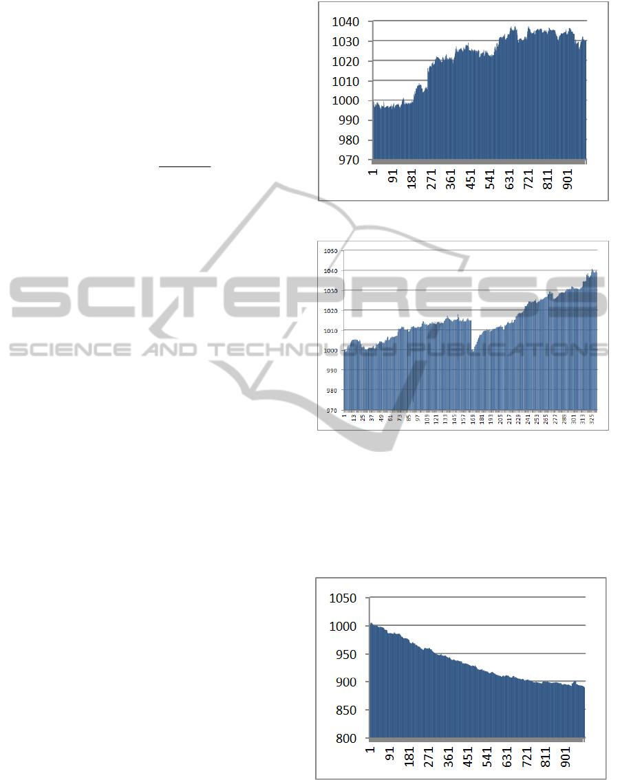
4.1 Prediction and Trading
on mid Price
As was mentioned before, in the first case we only
predict and trade on the mid-price. The results are
indicated by figures 4.1.1 and 4.1.2, respectively.
One can see that the we can achieve a 3 % or in
quantity profit= $30.29; Profit=3% ; MAX
Drawdown=0.5%.
One can see that the we can achieve a 3.9 % or in
quantity profit= $39.70; Profit=3.9%; MAX
Drawdown=0.24%.
Figure 4.1.1: Balance with respect to time (single asset).
Figure 4.1.2: Balance with respect to time (Portfolio).
4.2 Training on the mid Price
and Trading on Bid/Ask
In this case we use mid-price for prediction but we
trade on Bid/Ask. Here on horizontal axis we have
the same number of trades as in the previous figure.
Figure 4.2.1: Balance with respect to time (single asset).
The achieved profits are negative -10.70%,-5.8%
(Profit: -110.70$, -58$) MAX Drawdown=3.4%,
2.1%.
IJCCI2013-InternationalJointConferenceonComputationalIntelligence
504

Figure 4.2.2: Balance with respect to time (Portfolio).
The result is not so good as we have negative
balance growth on vertical axis. However, as
expected this is due to the fact we have not exploited
the information given in the bid and ask series.
4.3 Training on the Bid/Ask
and Trading on the Bid/Ask
In this case, we use following model to cover the
spread.
(y, x, w)
Bid
k
Netx
(4.9)
(y, x, u)
Ask
k
Nety
(4.10)
1kk
x
y
BUY
1kk
yx
SELL
In the figure bellow we have smaller number of
trades on horizontal axis in comparison to previous
cases because it might happen that the predicted
value is not greater than Ask Price or it is not even
less than Bid Price, therefore in some cases we do
not trade. Again on the vertical axis we have account
balance but this time we have some positive growth.
Figure 4.3.1: Balance with respect to time (single asset).
The achieved profit 1.23 %( Profit: $12.30)
which is good in the presence of bid-ask spread.
MAX Drawdown=0.85%. One can see that even
in the presence of bid-ask spread the method can
materialize profit.
Figure 4.3.2: Balance with respect to time (Portfolio).
The achieved profit is 1.48 %(Profit:$14.8)which is
good in the presence of bid-ask spread. Max
Drawdown=0.29%.
5 OPTIMIZING THE STEP
So far in our main model we only predicted the next
candle(time instant), but we can also predict more
than one candle. It can help us to better cover the
spread and possibly extend our profit, as we let the
price series change more dominantly to get out of
the spread and materializing more profit. Here our
goal is to find the optimal step parameter, where the
step is defined as how many candles in the future we
predict.
The next figure shows the result regarding the
step parameter, i.e. the account profit in percentage
(optimization period is 6 months) is plotted as a
function of the step parameter.
Figure 5.1: Profit as a function of prediction step.
From Figure 5.1, one can conclude that the optimal
step parameter is 7.
Predictionbased-HighFrequencyTradingonFinancialTimeSeries
505

6 CONCLUSIONS AND FURTHER
WORK
In this paper we used FFNN based prediction for
trading on financial time series. The optimal trading
strategy has been derived by using the fact that
FFNN can represent the conditional expected value.
Furthermore, we have optimized the prediction step
parameter numerically. In the case of trading on the
mid-price a considerable amount of profit can be
accumulated. In the case of trading in the presence
of bid-ask spread the method is still profitable but
the achieved profit is more modest.
The methods presented here can pave the way
towards high frequency, intraday trading.
Furthermore, in our tests we did not use leverage,
but with these low drawdowns which we had, we
can easily use bigger leverages to magnify our
profit. Although the ability to earn significant profits
by using leverage is substantial, leverage can also
work against investors. For example, if the currency
underlying one of the trades moves in the opposite
direction of what the investor believed would
happen, leverage will greatly amplify the potential
losses. To avoid such a catastrophe, Forex traders
usually use money management techniques.
ACKNOWLEDGEMENTS
The work reported in the paper has been partly
developed in the framework of the project „Talent
care and cultivation in the scientific workshops of
BME" project. This project is supported by the grant
TÁMOP - 4.2.2.B-10/1--2010-0009.
REFERENCES
A Hanif, R., 2012. Algorithmic, Electronic and Automated
Trading.
Box, G. E., Tiao, G.C. , 1977. A canonical analysis of
multiple time series.
D’Aspremont, A., 2011. Identifying small mean-reverting
portfolios.
J. W., 2002. Portfolio and Consumption Decisions under
Mean-Reverting Returns: An Exact Solution for
Complete Markets.
Kissell, R., 2006. Algorithmic trading strategies.
L., C., 2012. Predictability and Hedge Fund Investing..
Peter Bergan, C., 2005. Algorithmic Trading What Should
You Be Doing?.
Pole, A., 2007. Algorithmic trading insights and
techniques.
R. Balvers, Y. W., E Gilliland , 2000. Mean Reversion
across National Stock Markets and Parametric
Contrarian Investment Strategies.
R. L. Naik, D. R., B Manjula, A Govardhan, 2012.
Prediction of Stock Market Index Using Genetic
Algorithm.
Y. Zuo, E. K., 2012. Up/Down Analysis of Stock Index by
Using Bayesian Network.
IJCCI2013-InternationalJointConferenceonComputationalIntelligence
506
