Classification of Power Quality Considering Voltage Sags occurred in

Feeders

Anderson Roges Teixeira Góes

, Maria Teresinha Arns Steiner

2, 3

and Pedro José Steiner Neto

Graduate Programs in Numerical Methods in Engineering, Federal University of Paraná,

Centro Politécnico, CP: 19081, CEP: 81531-990, Curitiba, PR, Brazil

Graduate Program in Industrial and Systems Engineering, Pontifical Catholic University of Paraná,

Rua Imaculada Conceição, 1155, Prado Velho, CEP: 80.215-901, Curitiba, PR, Brazil

Graduate Programs in: Numerical Methods in Engineering and Industrial Engineering, Federal University of Paraná,

Centro Politécnico, CP: 1908, CEP: 81531-990, Curitiba, PR, Brazil

Graduate Programs in Business Administration, Federal University of Paraná,

Av. Pref. Lothario Meissner, 632 2º andar - Jardim Botânico, CEP: 80210-170, Curitiba, PR, Brazil

Keywords: EEQ Classification, Quality Label, KDD Process, Pattern Recognition, Real Case Study.

Abstract: In this paper we propose a methodology to classify Power Quality for feeders, based on sags and by the use

of KDD technique, establishing a quality level printed in labels. To support the methodology, it was applied

to feeders on a substation located in Curitiba, Paraná, Brazil, based on attributes such as sag length, duration

and frequency (number of occurrences on a given period of time). In the search for feeders quality

classification, on the Data Mining stage, the main stage on KDD process, three different techniques were

used in a comparatively way for pattern recognition: Artificial Neural Networks, Support Vector Machines

an Genetic Algorithms. Those techniques presented acceptable results in classification feeders with no

possible classification using a simplified method based on maximum number of sags. Thus, by printing the

label with information and Quality level, utilities companies can get better organized for mitigation

procedures, by establishing clear targets.

1 INTRODUCTION

Currently, is growing the consumer demand for

quality in both products & services provided,

because businesses in various industries have been

using high-sensitivity computerized equipment that

must rely on good Power Quality (PQ), and this has

been fostering several studies about PQ.

Many disturbances occur in the electric system,

usually called “events”, which can be either

accidental (tree branch fall, atmospheric discharges)

or programmed (preventive maintenance); such

events have a direct influence on PQ.

These events generate some PQ indicators or

continuity indicators (both individual and

collective), currently presented by Brazilian

concessionaires, who are related to Power outages,

but not present indicators concerning voltage sag.

In this context, this paper proposes a

methodology that could be considered an alternative

to the requirement made by Aneel (2008) that does

not define performance standards for the voltage sag

event but indicates that “concessionaires should

follow up and make available, on an annual basis,

the performance of monitored bus bars”. This

information could be a benchmark for bar

performance of consumer units serviced by the

Medium and High Voltage Distribution System with

sensitive loads and short-duration voltage variations.

The classification proposed hereby considers

only three attributes: voltage sag magnitude,

duration and frequency (number of events during a

certain period); this classification led to the creation

of a PQ label that classifies feeders according to a

six-color scale, where each color stands for a quality

level (from A to F, where A is the highest quality

and F is the lowest quality). In this paper, we

decided to present an illustration of the methodology

applied to feeders of a substation in the municipality

of Curitiba, Paraná, Brazil, which could be

generalized and applied to other issues (Góes, 2012).

The inspiration to create a quality label for

433

Teixeira Góes A., Arns Steiner M. and Steiner Neto P..

Classiﬁcation of Power Quality Considering Voltage Sags occurred in Feeders.

DOI: 10.5220/0004511104330442

In Proceedings of the 5th International Joint Conference on Computational Intelligence (NCTA-2013), pages 433-442

ISBN: 978-989-8565-77-8

 2013 SCITEPRESS (Science and Technology Publications, Lda.)

voltage sags came after a literature review of the

researches of Casteren et al., (2005) and Cobben and

Casteren (2006), who outlined a PQ classification,

however, without presenting a methodology or

techniques to make the PQ effective for voltage

sags.

Thus, as there seems to be no other studies

addressing PQ (only PQ-related events) in literature,

some topics in the studies by Casteren et al., (2005)

and Cobben and Castaren (2006) are analyzed here:

1. How to use real data in order to create a quality

label?

2. How to define what is “regular quality”, based

on real data?

3. How to classify an element/pattern that fits none

of the classification levels in the quality label?

The methodology present in this paper brings in its

context the Knowledge Discovery in Data bases

(KDD) to answer the questions above.

In the first question, we used a historical data

base of an electric power company from a substation

during a four-month period (February to May,

2008). The second question is answered by

achieving the upper limit of the “C” range, presented

throughout the paper. Finally, in order to answer the

third question, we used three pattern recognition

techniques: Artificial Neural Networks (ANN),

Support Vector Machines (SVM) and Genetic

Algorithm (GA), at the Data Mining stage (main

stage of the KDD process).

This paper is organized in five sections,

including the introduction. The literature review

indicating related studies to this theme. The problem

is described in section 3; section 4 presents the

methodology applied to a real problem addressed

here and, finally, section 5 presents the conclusions.

2 LITERATURE REVIEW

The research studies related to power network

disturbances (voltage sags, overvoltage, Total

Harmonic Distortion, frequency, unbalanced

circuits, among others) reunite many research

studies that use Operational Research techniques

aiming at their identification, location, classification

and prediction. Some of these research studies were

developed by Trindade (2005), Oleskovicz et al.,

(2006), Adepoju et al., (2007), Kaewarsa,

Attakitmongcol and Kulworawanichpong (2008),

Caciotta, Giarnetti and Leccese (2009), Gencer et

al., (2010), Kappor and Saini (2011) and Dash et al.,

(2012). However, most of them do not directly

address PQ classification; instead, as mentioned

above, they address disturbances affecting quality.

On the other hand, the literature has at least two

studies outlining PQ classification. One of them was

developed by Cobben and Castaren (2006) and it

presents three methods for PQ classification based

on: small voltage variations, voltage swings and

voltage drops; however, without clarifying the

methodology, thus leaving many gaps. These

classification methods match transparency and

simplicity once they use a classification system

based on a quality label as illustrated in Figure 1.

This illustration is from Casteren et al., (2005) – the

other study, which seeks to classify voltage sags as

to allow pointing the accountability (consumer,

equipment manufacturer or concessionaire) for the

cause of the event and its mitigation measures by

examining the duration and remaining value of such

sags.

Very high quality

High quality

Regular quality

Low quality

Very low quality

Extremely low quality

Figure 1: PQ label. Source: Casteren et al., (2005).

With this data in hand, Casteren et al., (2005)

outline a quality label according to frequency

(occurrences number), in order to classify sags

according to a table divided into nine different

levels, as shown in Figure 2, grouped into three

regions, where each region represents an

responsibility area.

500 ms 10 s 5 min

100%

90%

80%

70%

60%

50%

40%

30%

20%

10%

M0 L0

Figure 2: Voltage sag responsibility (duration x remnant

voltage). Source: Casteren et al., (2005).

The upper region (K0, M0, L0), with duration

varying between 500 ms and 5 min and remnant

voltage between 80% and 100%, is the

manufacturer’s responsibility. The intermediate

region (K1, M1, L1), with analogous interpretation,

IJCCI2013-InternationalJointConferenceonComputationalIntelligence

434

is the consumer’s responsibility area. Finally, the

lower region (K2, M2, L2) is the concessionaire’s

responsibility. The authors do not have any detailed

sag data, either measured or simulated; therefore, the

numbers presented in the presented standard criteria

are fictitious. Figure 3, for example, would indicate

that a consumer could annually experience a

maximum of five K1 sags, three M1 sags and L1

sags; any number above these would result in

penalties to the concessionaire. M2 sags are allowed

only once every two years.

The upper region (K0, M0, L0), with duration

varying between 500 ms and 5 min and remnant

voltage between 80% and 100%, is the

manufacturer’s responsibility. The intermediate

region (K1, M1, L1), with analogous interpretation,

is the consumer’s responsibility area. Finally, the

lower region (K2, M2, L2) is the concessionaire’s

responsibility. The authors do not have any detailed

sag data, either measured or simulated; therefore, the

numbers presented in the presented standard criteria

are fictitious. Figure 3, for example, would indicate

that a consumer could annually experience a

maximum of five K1 sags, three M1 sags and L1

sags; any number above these would result in

penalties to the concessionaire. M2 sags are allowed

only once every two years.

500 ms 10 s 5 min

100%

90%

80%

70%

60%

50%

40%

30%

20%

10%

0.8

0.5

0.2

- - -

- - - - - -

Figure 3: Example of a sag characterization criterion.

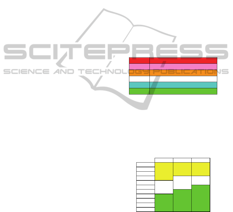
In order to facilitate communications between

consumers and concessionaires, the authors prepared

a PQ classification label (or quality label) based on

the sag characterization criteria, as shown in Figure

4. According to this classification, “A” indicates

high power quality and “E” means low power

quality.

Figure 4: Power quality label. Source: Casteren et al.,

(2005).

The PQ classification presented in Figure 4 must

be linked to the sag characterization criteria (Figure

3) and, therefore, the authors used the upper “C”

level limit criterion as shown in Figure 5, below.

Analogously, additional criteria tables can be created

to define the upper A, B and D limits.

The authors conclude that this classification

method is simple and consistent, as it requires only

multiplication factors, which are defined according

to the concessionaires’ criteria.

0.2 1

0.5 1.5

EABCD

- - -

- - - - - -

4.5

7.5

0.3

0.8

1.2

- - -

- - - - - -

1.5

2.5

0.1

0.3

0.4

- - -

- - - - - -

0.2

0.5

0.80.2

0.1

0,04

- - -

- - - - - -

0.6

Figure 5: PQ classification method (linking Figures 3 and

4).

However, some considerations made by the

authors are not so obvious and it seems that the

literature does not have other studies answering the

questions made in section 1: how to use real data to

create a quality label? How to define what is

“regular quality” based on real data? How to classify

an element that does not fit any classification range

in the quality label such as, for example, K1, K2,

M1 and L1 pertaining to the values in the “B”

classification range, when M2 and L2 have values in

the “D” classification range (Figure 6)?

500 ms 10 s 5 min

100%

90%

80%

70%

60%

50%

40%

30%

20%

10%

0.25

0.19

0.29

- - -

- - - - - -

1.1

2.3

Figure 6: Example of sag events that do not fit the

framework of Figure 5.

Thus, for element classification, as shown in

Figure 6 above, we used the KDD process (Góes,

2012).

ClassificationofPowerQualityConsideringVoltageSagsoccurredinFeeders

435

3 PROBLEM DESCRIPTION

With the purpose of achieving the first objective of

the research, which consists in using real data to

indicate the PQ, data were collected from a power

company for application of the methodology

developed. This company supplies 399

municipalities and 1,114 localities (districts, small

towns and villages) in the State of Paraná in Brazil.

At the time of the survey, it had 378 substations (SS)

in order to supply around four million consumers

(households, industries and others); specifically in

the capital city, there were 30 substations with

around 300 feeders (approximately 10 feeders per

SS).

In 14 of the 378 substations, a device is installed

to detect PQ-events also measuring voltage sags. Of

these 14 devices, six devices are installed in

substations in the capital city and its metropolitan

area.

The methodology proposed in the present study

is applied to one of these substations, which is

composed of 12 feeders. However, it should be

noted that this methodology can be applied to any

substation as long as it has a data collector to capture

the information required.

The historical records of events (voltage sags)

required to develop the proposal of this study are

stored in the concessionaire’s data bases. In the first

data base, here called BD01, data are captured by the

device installed in the bus bar of the substation.

Each of these records contains 17 data (attributes),

namely: “oscillographic identification”, which

consists in record numbering by the concessionaire

software; “date and time of event start”, which

indicates the initial time of the PQ-related event

record; “type of event”, which indicates the PQ-

related phenomenon: voltage sag or voltage swell,

among others; and “remnant voltage or root mean

square (RMS)”, which indicates the remnant

voltage, that is, the voltage “left” after the event

occurrence at each of the voltage phases (Phase A,

Phase B and Phase C).

The records in the second data base, BD02, are

captured by the concessionaire’s Distribution

Operation System (DOS) and are related to the

interruptions. These records, obtained through

software developed by the concessionaire, supply 29

attributes, among which: “feeder identification” –

feeder name of the power grid where the interruption

was generated; “data and time of event onset” –

moment when the interruption occurred; “duration”

– interruption duration; “type” - description of

interruption type (accidental, programmed or

voluntary) and “component affected” – description

of the electrical component affected.

The data used in the study was collected during a

four-month period, between February and May

2008; the BD01 was formed by 352 records and the

BD02 was formed by 422 records. Thus, a procedure

is necessary to analyze and explore this information,

transforming it into knowledge. This will require the

use of the KDD process aiming at data exploration

that will ultimately produce the PQ label.

4 METHODOLOGY

APPLICATION

The KDD process was used as the foundation of the

methodology developed here to produce the PQ

label. This process is composed for five steps: data

selection; data preprocessing; data transformation;

data mining and, finally, interpretation of the

knowledge generated (Fayyad et al., 1996). But in

this paper the KDD process that is basically

composed of the following stages: data

preprocessing (data cleaning and transformation);

data association between data bases (BD01 and

BD02) and, finally, the creation of the label itself. At

the last stage, Data Mining techniques were used in

order to achieve pattern recognition: ANN; AG and

SVM, as already commented. (Góes, 2012)

4.1 Data Pre-processing

At this stage of the KDD process, the attributes

relevant to the study were analyzed; eight attributes

were removed from BD01 and nine attributes were

left (described in the section 3 above). With regard

to the BD02 preprocessing, the number of attributes

was reduced to six for the same reason (also

described above).

Also, only the records where “Type” attributes

were “Accidental” should be considered, for the

others “Types” it is possible to monitor PQ

disturbances. As this information is present

exclusively in BD02, this data base was filtered

again, after which only five attributes were left, thus

also reducing the numbers of records from 422 to

181.

Transformation of attributes that indicate

remnant voltage at each of the voltage phases was

performed, called “aggregation of parameters”, that

is, the remnant voltage of the event was defined as

the lowest value among the values achieved by the

three voltage phases – an alternative indicated by

Aneel (2008). Event duration, in turn, is defined as

the maximum duration between the three

IJCCI2013-InternationalJointConferenceonComputationalIntelligence

436

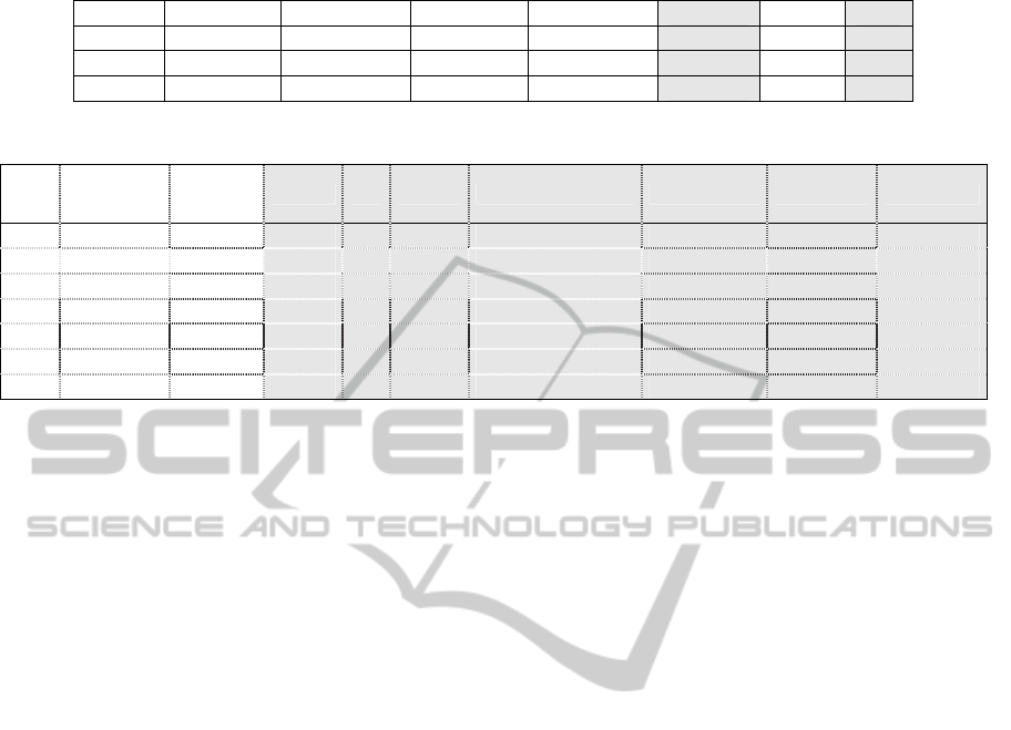
Table 1: Some BD01 records after data transformation.

Id. Osc. Start Date Start Time Final Date Final Time

Duration Circuit RMS

9 2008-02-06 07:28:35.034 2008-02-06 07:28:35.252 218 0 60.1

10 2008-02-06 20:04:14.805 2008-02-06 20:04:14.990 185 1 35.9

... ... ... ... ... ... ... ...

Table 2: Examples of BD03 records (association between BD01and BD02).

Id.

Osc.

Start Date Start Time

Duration RMS Feeder Component Affected Start Date Start Time Duration

117 28/04/2008 14:28:43 185 46.3 AC Fly tap 28/04/2008 14:30 135

117 28/04/2008 14:28:43 185 46.3 AF AR actuation 28/04/2008 14:29 1

117 28/04/2008 14:28:43 185 46.3 AF Fusible link act. 28/04/2008 14:42 41

121 28/04/2008 18:07:50 202 42.6 AC Conductor - AT 28/04/2008 18:32 344

121 28/04/2008 18:07:50 202 42.6 AI Conductor - BT 28/04/2008 18:16 403

136 02/05/2008 7:13:10 705 28.7 AF Pole 02/05/2008 07:15 36

139 08/05/2008 11:13:04 168 42.4 AI AR actuation 08/05/2008 11:14 0

phase/neutral events. These values were recorded in

the new “Remnant voltage” attribute, and the “RMS

voltage phase A”, “RMS voltage phase B” and

“RMS voltage phase C” attributes were excluded

from BD01.

The methodology proposed to create the PQ

label of a feeder considers only three attributes:

remnant voltage, duration and number of

occurrences. The first two attributes are in BD01

(Table 1); the third attribute is the result of a simple

occurrence count. However, BD01 does not indicate

the feeder that was affected by the event as data

relative to feeders are present in BD02.

Thus, it is necessary to associate BD01 records

with BD02 records, according to a procedure

presented in the next section.

4.2 Data Association (BD01 and BD02)

In order to associate the date contained in BD01 and

BD02, attributes related to time were used. More

specifically, “Start Date” and “Start Time” attributes

in BD01 and “Start Date” and “Start Time”

attributes in BD02 were used.

This association generated a new data base,

called BD03, containing 169 records. That is, of the

352 records in BD01 and the 181 records in BD02,

there are 169 records associated according to the

criterion above.

Table 2, with 10 columns, presents some

examples/records of this association. The

information in columns 1 to 5 is data from BD01

while columns 6 to 10 are their respective

associations found in BD02. In addition, as a means

of identifying the 12 feeders in this substation, they

will be generically called AA, AB, AC,..., AK, and

AL.

Table 2 shows that one record in BD01 may have

more than one association with BD02, as in the case

of the first three lines of the table, where the

“Oscillography Identification” attribute is 117. This

indicates that the event captured in the substation

was also “captured” or was originated in two

feeders, “AC” and “AF”, where “AF” has two

records for different components affected: “Fly

Tap”, “AR actuation”, or simply “AR” and “Fusible

link actuation”.

4.3 Creating the PQ Label for the

Feeders

The classification of each BD03 record started with

the construction of a classification table (Table 3)

inspired by the proposal made by Casteren et al.,

(2005), as shown in section 2.1, with the following

attributes: remnant voltage, duration and number of

events. The division proposed in this paper for the

table was made as follows: two duration ranges were

considered for the event: ≤ 500 and > 500

milliseconds and five remnant voltage intervals:

10% to 19%, 20% to 39%, 40% to 59%, 60% to

79% and 80% to 90%.

The connection between duration and remnant

voltage can be better understood by observing Table

3, where 10 possible classes, called C1, C2,... to

C10,, are presented. It becomes evident that, the

shorter the duration, the higher the remnant voltage

of the event, and the better the PQ of that event will

be. Thus, the PQ of events has the following

hierarchy: C1 ≥ C2 ≥ ... ≥ C10. In order to typify

such classification, records in Table 2 are duly

classified, according to Table 3 and Table 4.

ClassificationofPowerQualityConsideringVoltageSagsoccurredinFeeders

437

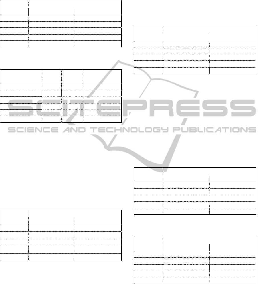
Table 3: Classification considering duration and remnant

voltage in the records.

RMS (%)

Duration

≤ 500 milliseconds > 500 milliseconds

80 to 90% C1 C2

60 to 79% C3 C4

40 to 59% C5 C6

20 to 39% C7 C8

10 to 19% C9 C10

Table 4: Classification of records in Table 2 according to

Table 3.

Duration

(milliseconds)

RMS

(%)

Feeder

Record

Classification

185 46.3 AC C5

185 46.3 AF C5

202 42.6 AC C5

202 42.6 AI C5

705 28.7 AF C8

By defining this classification for the 169 BD03

records do BD03, the “AA” feeder record numbers,

for example, are those presented in Table 5. Record

classification is obtained similarly for the other

feeders in the substation. Table 5 shows that the

“AA” feeder has two events of the C5 type: one of

the C7 type and one of the C8 type. Considering all

the 169 records of all the 12 feeders in the

substation, Table 6 shows that only three of those

ranges have records: C5, C7 and C8.

Table 5: Classification of voltage sags of the “AA” feeder.

RMS (%)

Duration

≤ 500 milliseconds > 500 milliseconds

80 to 90% 0 0

60 to 79% 0 0

40 to 59% 2 0

20 to 39% 1 1

10 to 19% 0 0

In order to obtain the “average quality” of the

substation under analysis, the number of events in

Table 6 was divided by 12 (total feeders), obtaining

the data in Table 7, already duly rounded.

Therefore, in order to create the PQ label, the

values of six ranges were established, where “Range

A” is the best PQ and “Range F” is the worst one.

For each range factors – defined in conjunction with

the concessionaire’s engineers - were multiplied to

determine the upper limit of each range. Thus,

Table 7 above represents the feeder average, that is,

the upper limit of “Range C”. The upper bound of

“Range A” (Table 8) was obtained by multiplying

values in Table 7 by 0.25.

Table 6: Classification of voltage sags in the substation

analyzed considering all the records.

RMS (%)

Duration

≤ 500 milliseconds > 500 milliseconds

80 to 90% 0 0

60 to 79% 0 0

40 to 59% 149 0

20 to 39% 15 5

10 to 19% 0 0

The upper bound of “Range B” was obtained by

multiplying the values in Table 7 by 0.50. By

multiplying the values in Table 7 by 1.5, the upper

bound of “Range D” was obtained. The upper bound

of “Range E” was obtained by multiplying the

values in Table 7 by a 2.0 factor. Finally, the upper

bound of “Range F” was obtained by verifying the

highest value presented for the feeders under

analysis. These values are presented in the PQ

classification label (Figure 7).

Table 7: Average classification of voltage sags in the

substation analyzed.

RMS (%)

Duration

≤ 500 milliseconds > 500 milliseconds

80 to 90% 0 0

60 to 79% 0 0

40 to 59% 13 0

20 to 39% 2 1

10 to 19% 0 0

Table 8: Upper bound of “Range A” in the PQ

classification label of a feeder in a particular substation.

RMS (%)

Duration

≤ 500 milliseconds > 500 milliseconds

80 to 90% 0 0

60 to 79% 0 0

40 to 59% 4 0

20 to 39% 1 1

10 to 19% 0 0

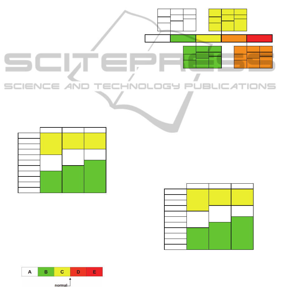
Once the label is created, the classification of

each feeder only requires verifying which range

interval presented in Figure 7 the feeder fits in.

IJCCI2013-InternationalJointConferenceonComputationalIntelligence

438

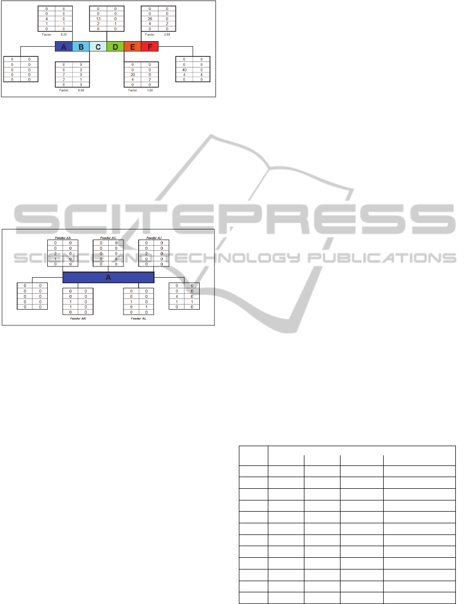
Figure 7: PQ classification label of feeders in a particular

substation.

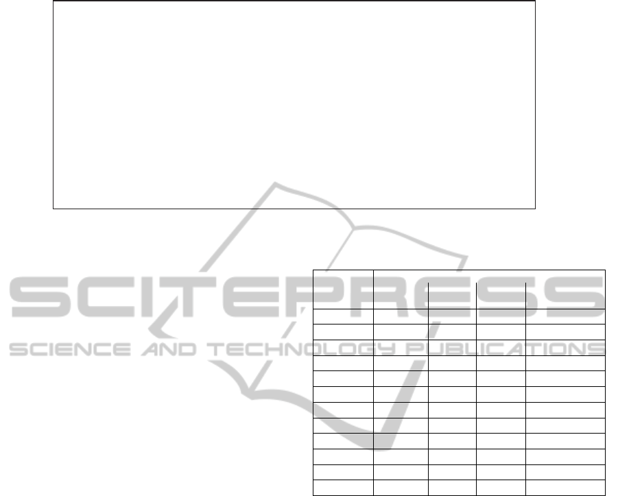
However, it becomes evident that such task is not

so simple, as only five of the 12 feeders fit in these

range of values, all of them with and “A” quality

classification, namely: AA, AG, AJ, AK and AL.

The five feeders present values for C5 pertaining to

the [0, 4] interval and for C7 and C8, in the [0, 1]

interval, as illustrated in Figure 8.

Figure 8: Feeders classified directly from the PQ label.

Other feeders could not be directly classified as,

for example, for feeder AH the value of C5 equals

16, which indicates that its classification would be

D. However, in this feeder, C7 and C8 are outside D

class intervals. Thus, in order to classify the other

feeders, we used three Data Mining techniques,

comparatively.

4.4 Data Mining Techniques

The DM stage is the most important stage in the

KDD process, as it is the moment when pattern

recognition techniques are applied, either through

heuristic or through metaheuristic procedures. In this

study, such procedures are applied aiming at the PQ

classification of feeders in a substation.

In this paper we present the application three

techniques used to classify feeders that could not be

directly classified. Her particularities can be seeing

in Góes (2012).

4.4.1 Artificial Neural Networks

In the ANN (Haykin, 1999) application, the

backpropagation learning algorithm was used, which

was implemented in Visual Basic 6.0. Each ANN

trained had three inputs (C5, C7 and C8) for the

input layer, hidden layer (with number of neurons

varying between “1” and “20”) and one neuron in

the output layer (to indicate the class). The sigmoid-

logistic function is the activation function for all

(hidden and output layers).

The network was trained five times; the initial

weight set varied at random in the (-1,1) interval.

There were 1,500 tests in total (3 stages x 5 initial

weight sets x 20 quantities of neurons in the hidden

layer x 5 classification ranges). The training was

completed when one of the following conditions was

met: 1,000 iterations; mean square error less than or

equal to 10-4; or a number of records incorrectly

classified as equal to zero. Regarding the problem

approached here, the percentage of correctness in the

training of this technique was 99.88%, considering

the three stages of the three-fold method, and

99.67% in the test. Table 9 below presents the feeder

classification results achieved with the application of

this technique. In Table 9, as well as with the others

to be presented, the “Voting Classification” column

(last column) indicates the classification with

highest occurrence in the former columns, that is,

the statistical mode.

In spite of the fact that AA, AG, AJ, AK and AL

feeders already have their classification defined, as

they were directly classified in the quality label, they

were also introduced to the networks, thus

confirming classifications. Therefore, six feeders

had “A” classification, one feeder had “B”

classification, two feeders had “C” classification,

one feeder had “D” classification, one feeder had

“E” classification and one feeder had “F”

classification.

Table 9: Feeder classification results – ANN.

Feeder

Stratified Three-fold Procedure

stage 2

tage 3

stage Voting Classificat.

A A A A

C C C C

D D D D

C C B C

B B B B

F F F F

A A A A

E E E E

A A A A

ClassificationofPowerQualityConsideringVoltageSagsoccurredinFeeders

439

Define P

= [X(1) X(2) X(3)]; P

= [X(4) X(5 X(6)]; P

= [X(7) X(8) X(9)].

Determine the plane



equation that contains P

, P

and

For each element k

Replace variables in plane



equation with k values, obtaining the variable Value.

Calculate the Euclidian distance between k and



, obtaining the variable Dist.

If k

CL1, then

If Value < 0, then correct = correct+1;

If Dist01 > Dist, then Dist01= Dist;

If k

CL2, then

If Value > 0, then correct = correct+1;

If Dist02 > Dist, then Dist02 = Dist;

z1= correct / number of examples k;

z2=module (Dist01 – Dist02) * penalty;

Fitness of X = z1 - z2.

Figure 9: Pseudocode for fitness calculation.

4.4.2 Support Vector Machines

As to the SVM (Vapnik, 1995); (Burges, 1998) at

first the svmtrain function of Matlab 7.9.0 was used

with two matrices in the arguments: Examples and

Answers, according to the equation (1).

Training = svmtrain(Examples,Answer) (1)

The “Examples” matrix has in their columns the Ci

values and the “Answers” matrix has only one

column with the range value that each pattern

(“Examples” matrix line) has as its answer.

Subsequently, the test set was used, described here

in the form of matrix, named “New”, and the result

of “Training” with the svmclassify function,

equation (2), with the purpose of verifying the

percentage of correct classification of the new data.

Classification = svmclassify(Training,New) (2)

It should be noted that the arguments used in the

training for the svmtrain function are default for

Matlab 7.9.0, as the range sets of the quality label

are linearly separable by a plane. In this technique,

15 tests (3 training stages x 5 classification ranges)

were carried out. The percentage of correctness in

the training of this technique was 100%, considering

the three stages of the three-fold procedure, and it

was 99.55% in the test. Table 10 below presents the

result of feeder classification achieved with the

SVM application.

Table 10 indicates that the feeder voting

classification is: seven with “A” classification, none

with “B” classification, and three with “C”

classification, none with “D” classification, one with

“E” classification and one with “F” classification.

This technique also correctly classified AA, AG, AJ,

AK and AL feeders, which were directly classified

in the quality label.

Table 10: Feeder classification results – SVM.

Feeder

Stratified Three-fold Procedure

stage

Voting

Classificat.

A A A A

C C C C

D C C C

C C B C

A A A A

F F F F

A A A A

D E E E

A A A A

4.4.3 Genetic Algorithm

The GA (GOLDBERG, 1989) was used with the

purpose of determining a plane so that each one of

the resulting half-spaces contained only one of the

sets of each application stage, according to aspects

highlighted in the beginning of section 4.4. The

value of the fitness functions is established by an

algorithm that determines three points defining such

plane, where the coordinates of each point are

individuals’ alleles.

Each individual is composed of nine alleles with

values belonging to the set of real numbers. Thus,

the first three alleles represent the coordinates of a

P1 point, the next three alleles are coordinates of the

P2 point, and the last three alleles are coordinates of

the P3 point. There is also the fitness calculation that

takes into account the difference of the distance

between two points (in different sets) closer to the

plane determined. The greater the difference

between distances, the greater is the penalty in

fitness. Therefore, Figure 9 presents this algorithm,

where X is a vector in which each coordinate

IJCCI2013-InternationalJointConferenceonComputationalIntelligence

440

represents an allele of the population’s individual;

CL1 and CL2 are training sets and k is an element

pertaining to CL1

 CL2.

In order to apply the GA, the 0.1 “penalty” and

the Matblab 7.9.0 toolbox – gatool - were used. The

arguments for the training were the default that

achieved the best results. In one population type, the

Double Vector - where each allele is a real number –

was used.

Table 11: Feeder classification result – AG.

Feeder

Stratified Three-fold Procedure

stage 2

stage 3

stage Voting Classificat.

A A A A

E C C C

B B C B

A A A A

F F F F

A A A A

E C C C

A A A A

The percentage of correctness in the training was

100%, considering the three stages of the three-fold

method, and 99.11% in the test. Table 11 below

presents the feeder classification result achieved

through the application of this technique. Here, the

AA, AG, AJ, AK and AL feeders also confirmed the

classifications previously achieved. Thus, there are

six feeders with “A” classification, one feeder with

“B” classification, four feeders with “C”

classification, no feeder with “D” classification, no

feeder with “E” classification and one feeder with

“F” classification.

5 RESULT ANALYSIS AND

CONCLUSIONS

The analysis of results is the last stage in the KDD

process and is performed here by comparing

classifications obtained with the three techniques

applied. Table 12 presents the classification result

achieved (“voting classification” column in Tables 9

to 11). In addition, in this table there is also a

column named “voting classification” that indicates

the result with the highest occurrence among the

three techniques, which this analysis assumes as the

most adequate to the problem.

An analysis of Table 12 indicates that, among

the 12 feeders, seven feeders (AA, AB, AF, AG, AJ,

AK and AL) have the same classification under all

the techniques.

Table 12: Comparison between classifications achieved

through ANN, SVM and AG.

Feeder

Stratified Three-fold Procedure

ANN SVM AG

Voting

A A A

C C C

D C C

C C B

B A A

F F F

A A A

A A C

E E C

A A A

After a comparison between each technique and

the classification admitted as adequate (“voting

classification” column), the GA technique presents

three feeders (AD, AH and AI) with distinct

classifications, in two non-neighbor ranges.

According to this technique, the AD feeder has C

classification and the adequate classification is A;

the AI feeder was classified as C by AG, and E was

adequate. For the latter, the result presented by AG

is very distant from that of the other two techniques,

which presented the same result as the adequate

classification.

In the classification presented by the ANN

technique there are two feeders (AC and AE) with a

classification different from that presented in the

“voting classification”, but in neighbor

classification. For the AC feeder, the adequate

classification is C and ANN classified it as D, and

the AE feeder was classified by ANN as being B and

the adequate classification indicates A. Finally, the

SVM technique yields a result that is identical to the

“voting classification” column, which makes it the

most adequate technique for this case study.

Thus, the adequate feeder classification resulted

in seven feeders with “A” classification, no feeder

with “B” classification, three feeders with “C”

classification, no feeder with “D” classification, one

feeder with “E” classification and one feeder with

“F” classification (Figure 10).

In Figure 10, the values presented for each feeder

express event occurrence in each of the C5, C7 and

C8, classes in this order.

The label presents non-explicit knowledge when

ClassificationofPowerQualityConsideringVoltageSagsoccurredinFeeders

441

analyzing values such as, for example, classification

of AI and AF feeders, as C5 and C7 values in AI

area higher than in AF, which could indicate a lower

quality in AI compared to AF but, as C8 has a lower

value for AI, the techniques applied indicated that

AF has lower quality than the AI feeder.

Figure 10: Quality label with feeder classification.

Thus, the methodology developed and applied in

this study revealed non-explicit knowledge in the

concessionaire’s data bases to an unprecedented real

problem: the PQ considering voltage sags.

ACKNOWLEDGEMENTS

This study is an integral part of the P & D project

number 2866-019/2007 – Event Classification for

Power Quality, approved by ANEEL and developed

in partnership with COPEL and the UFPR.

REFERENCES

Adepoju, G. A.; Ogunjuyigbe, S. O. A.; Alawode, K. O.

Application of Neural Network to Load Forecasting in

Nigerian Electrical Power System. The Pacific

JouANNl of Science and Technology. Spring. v. 8, p.

68-72, 2007.

ANEEL Agência Nacional de Energia Elétrica.

Procedimentos de Distribuição de Energia Elétrica no

Sistema Elétrico Nacional – PRODIST: Módulo 8 –

Qualidade da Energia Elétrica. 2008.

Burges, C. J. C. A Tutorial on Support Vector Machines

for Pattern Recognition. Data Mining and Knowledge

Discovery, v. 2, p. 121-168, 1998.

Caciotta, M.; Giarnetti, S.; Leccese, F. Hybrid Neural

Network System for Electric Load Forecasting of

Telecomunication Station. XIX IMEKO World

Congress - Fundamental and Applied Metrology.

Lisboa, Portugal, p. 657-661, 2009.

Casteren, J. F. L. Van.; Enslin, L. H. R.; Hulshorst, W. T.

J.; Kilng, W.L.; Hamoen, M. D.; Cobben, J. F. G.

Acustomer oriented approach to the classification of

voltage dips. In: The18th International Conference

and exhibition on Electricity Distribuion – CIRED,

2005.

Cobben, J. F. G.; Casteren, J. F. L. Classification

Methodologies for Power Quality. Electrical Power

Quality & Utilization Magazine. v. 2, no 1, p. 11-17,

2006.

Dash, P. K.; Padhee, M.; Barik, S. K. Estimation of power

quality indices in distributed generation systems

during power islanding conditions. Electrical Power

and Energy Systems, v. 36, p. 18-30, 2012.

Fayyad, U.; Piatetsky-Shapiro, G.; Smyth, P.;

Uthurusamy, R. Advances in Knowledge Discovery &

Data Mining. 1 ed. American Association for Artificial

Intelligence, Menlo Park, Califórnia, 1996.

Gencer, O.; Ozturk, S.; Erfidan, T. A new approach to

voltage sag detection based on wavelet transform.

Electrical Power and Energy Systems, v. 32, p. 133-

140, 2010.

Góes, A. R. T. Uma metodologia para a criação de

etiqueta de qualidade no contexto de Descoberta de

Conhecimento em Bases de Dados: aplicação nas

áreas elétrica e educacional. 145 f. Tese (Doutorado

em Métodos Numéricos em Engenharia) - Setor

Tecnologia e Setor de Ciências Exatas, Universidade

Federal do Paraná, Curitiba, 2012.

Goldberg, D. E. Genetic algorithms in search, optmization,

and machines learning. Addison-Wesley Publishing

Company, Inc. Massachusetts, 1989.

Haykin, S. Neural Networks – A Comprehensive

Foundation. 2.nd., Prentice Hall, New Jersey, 1999.

Kaewarsa, S.; Attakitmongcol, K.;

Kulworawanichpong, T. Recognition of power quality

events by using multiwavelet-based neural networks.

Electrical Power and Energy Systems, v. 30, p. 245-

260, 2008.

Kappor, R.; Saini, M. K. Hybrid demodulation concept

and harmonic analysis for single/multiple power

quality events detection and classification. Electrical

Power and Energy Systems, v. 33, p. 1608-1622, 2011.

Oleskovicz, M.; Coury, D. V.; Carneiro, A. A. F. M.;

Arruda, E. F.; Delmont, O.; Souza, S. A. Estudo

comparativo de ferramentas modeANNs de análise

aplicadas à qualidade da energia elétrica. Revista

Controle & Automação, v. 17, n. 3. Julho, agosto e

setembro 2006.

Trindade, R. M. Sistema Digital de Detecção e

Classification de Eventos de Qualidade de Energia.

114 f. Dissertação (Mestrado em Engenharia Elétrica)

– Faculdade de Engenharia da Universidade Federal

de Juiz de Fora, Juiz de Fora, 2005.

Vapnik, V. The nature of statistical learning theory.

Springer-Verlag, New Yourk, 1995.

IJCCI2013-InternationalJointConferenceonComputationalIntelligence

442