Towards a Standard Approach for Optimization

in Science and Engineering

Carlo Comin, Luka Onesti and Carlos Kavka

Research and Development Department, ESTECO SPA, Area Science Park, Padriciano 99, Trieste, Italy

Keywords: Optimization, BPMN 2.0, Scientific Workflows, Simulation.

Abstract: Optimization plays a fundamental role in engineering design and in many other fields in applied science. An

optimization process allows obtaining the best designs which maximize and/or minimize a number of

objectives, satisfying at the same time certain constraints. Nowadays, design activities require a large use of

computational models to simulate experiments, which are usually automated through the execution of the

so-called scientific workflows. Even if there is a general agreement in both academy and industry on the use

of scientific workflows for the representation of optimization processes, no single standard has arisen as a

valid model to fully characterize it. A standard will facilitate collaboration between scientists and industrial

designers, interaction between different fields and a common vocabulary in scientific and engineering

publications. This paper proposes the use of BPMN 2.0, a well-defined standard from the area of business

processes, as a formal representation for both the abstract and execution models for scientific workflows in

the context of process optimization. Aspects like semantic expressiveness, representation efficiency and

extensibility, as required by optimization in industrial applications, have been carefully considered in this

research. Practical results of the implementation of an industrial-quality optimization workflow engine

defined in terms of the BPMN 2.0 standard are also presented in the paper.

1 INTRODUCTION

Optimization is the process of finding the best

solution for a problem given a set of restrictions or

constraints. Typical problems faced nowadays in

engineering and applied sciences, both in research

and industry, are defined with multiple and possibly

conflicting objectives. This class of problems,

known as Multi-Objective Optimization (MOO)

problems, usually do not have a single solution, but

a set of trade-off solutions where no objective can be

enhanced without a deterioration of at least one of

the others. This set of compromise solutions, known

as Pareto front, represents the output of an MOO

process (Branke et al., 2008).

Formally, an MOO problem is defined as

follows:



























,









,…,























0,  1,2,…,











0,  1,2,…,

where k is the number of objective functions, m is

the number of inequality constraints and e is the

number of equality constraints. The vector ∈



is

the vector of design variables while F corresponds

to the objective vector function.

In most engineering and applied sciences

problems, the objective vector function F represents

a physical problem, which is usually evaluated by a

so-called solver defined in terms of simulated

processes running on computer systems. This

computational process can be rather complex,

involving a large number of simulation steps, which

need to exchange data between themselves and can

require execution on distributed systems like a Grid

or Cloud Computing system. The simulated process

is usually represented with a formalism known as a

scientific workflow (Lin et al., 2009), which

provides both a representation for the abstract view

(used by the engineer to represent the process) and

the associated execution model (used for the real

simulation). The abstract view is usually a human-

understandable graphic representation, while the

execution model is usually represented with XML.

This last model is used by a workflow engine in

order to execute the workflow and perform the

simulation.

However, even if scientific workflows have been

169

Comin C., Onesti L. and Kavka C..

Towards a Standard Approach for Optimization in Science and Engineering.

DOI: 10.5220/0004490501690177

In Proceedings of the 8th International Joint Conference on Software Technologies (ICSOFT-EA-2013), pages 169-177

ISBN: 978-989-8565-68-6

 2013 SCITEPRESS (Science and Technology Publications, Lda.)

used successfully since many years, most of the

tools used for their definition and execution are not

based on standard technologies. A large number of

different graphic and execution formats are currently

in use, and there is no clear signs of convergence till

now. However, things are different in the area of

business processes, where many standards have

been defined for both the graphical and the

execution representation of business process

workflows. It is definitely true that most of the

business process standards cannot be used to

represent scientific workflows since they lack

enough expressive power to support specific

scientific workflow requirements. However, the

recent BPMN 2.0 (OMG, 2011) standard allows the

support of required characteristic for scientific

workflows at both levels, particularly due to its

powerful extension scheme, which can be used to

define the missing features. From now on, all

references with the acronym BPMN are intended as

references to version 2.0 of the standard.

While it is mostly accepted that BPMN can be

used to represent scientific workflows, this paper

will go one step forward. It will show that BPMN

can be used to represent a complete optimization

workflow, which includes not only the scientific

workflow used to represent the physical problem,

but also the optimization cycle supporting the

multiple patterns required by current optimization

problems. In this way, BPMN is opening the path for

the use of a single standard in optimization

workflows for engineering and applied science

applications, both in research and industrial fields.

The paper is structured as follows: Section 2

presents a short review of the state of the art, Section

3 describes optimization problems and the most

common optimization patterns in use today, Section

4 presents our proposal for the use of a standard

notations for optimization workflows and Section 5

presents results on a standard implementation by

considering specific requirements like execution

efficiency. The paper ends with conclusion and

references.

2 STATE OF THE ART

The use of scientific workflows for process

automation has been widely analyzed in the

literature (Lin et al., 2009). Many commercial and

open source implementations do exist. The most

widely used are Kepler (Ludascher et al., 2009),

Triana (Taylor et al., 2007), Taverna (Missier et al.,,

2010), Pegasus (Sonntag et al., 2010) and KNime

(Berthold et al, 2008), with many new frameworks

appearing continually. However, all these scientific

workflow frameworks are based in proprietary non-

standard formats. Attempts have been made to

represent scientific workflows by using standards;

for example, BPEL was proposed as the execution

representation for workflows using other models for

graphical representation, like BPMN or Pegasus

(Sonntag et al., 2010). However, the need to use two

different models, one for the abstract or graphical

representation, and the other for the execution

representation, prevented its widespread use in

industry.

Standards coming from the business process

area, like BPEL and the first version of BPMN had

some strong limitations to support all required

features. The latest release of the BPMN standard,

however, has open the possibility to use a single

standard in the context of scientific workflows due

to its powerful extension mechanism (Abdelahad et

al., 2012), even if in some cases the development

efforts can be important (Sonntag et al., 2010).

Concerning optimization workflows, there are

specific workflow systems defined for optimization

and also extensions of the previously mentioned

frameworks which can include optimization

components in them. As an example from the open

source community, Kepler through its module

Nimrod/OK, provides the possibility of defining

optimization cycles (Abramson, 2010). In the area of

commercial tools, there exists many options like for

example modeFRONTIER (ESTECO, 2012), widely

used in CAD/CAE engineering optimization.

However, again, all of them are based in proprietary

formats.

To the best of our knowledge, no current tool,

open source or commercial, can define optimization

workflows by using a standard workflow notation.

3 OPTIMIZATION PROBLEMS

An optimization session is defined through what is

usually know as an optimization plan (OP), which

consists at least in the specification of the design of

experiments strategy and the selection of the

optimization algorithm. Other elements, like robust

sampling or response surface models are usually

required in industrial applications (Branke et al.,

2008). The following subsections provide a short

description of these elements, together with an

specification of the most common optimization

patterns in use today.

ICSOFT2013-8thInternationalJointConferenceonSoftwareTechnologies

170

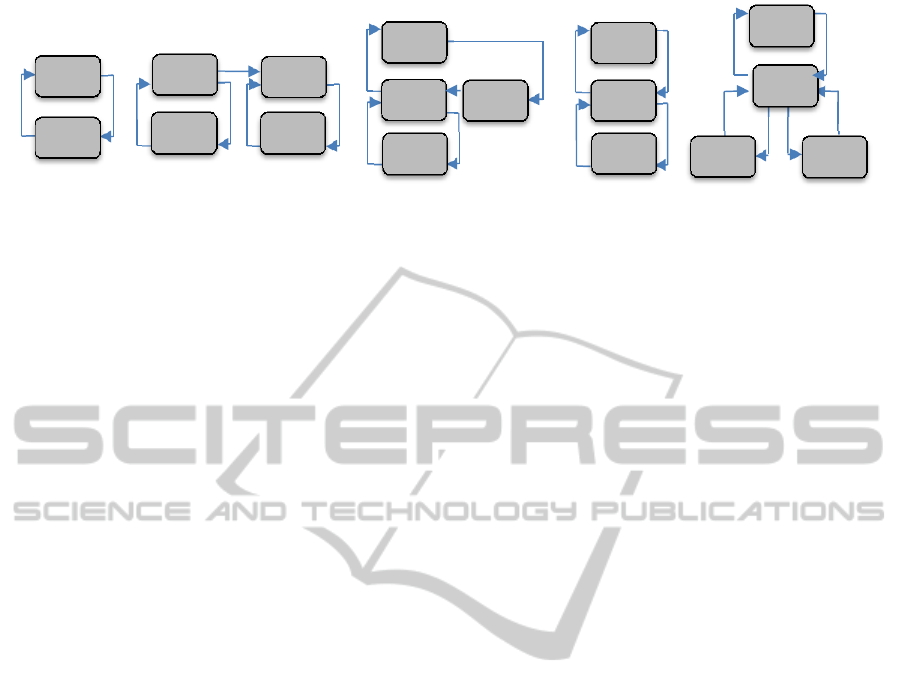
Figure 1: The most common optimization patterns: (a) simple, (b) sequential, (c) nested, (d) robust and (e) mixed robust.

3.1 Design of Experiments

A Design of Experiments (DoE) session usually

precedes the optimization stage. The aim of a DoE is

to test specific configurations regardless of the

objectives of the optimization run, but rather

considering their pattern in the input parameters

space. It provides an a-priori exploration and

analysis which is of primary importance when a

statistical analysis has to be performed later on.

Moreover, most optimization algorithms require a

starting population of designs to be considered

initially, eventually generating random input values

if no other preference has emerged yet.

3.2 Optimization Algorithms

The Optimization Algorithm (OA) implements the

mathematical strategies, or heuristics, which are

designed to obtain a good approximation of the

actual Pareto front. It is important to stress that real-

world optimization problems are solved through

rigorously proven converging methodologies only in

a very few cases, since the high number of input

parameters and the low smoothness of objective

functions involved limit the possible usage of

classical mathematical algorithms.

In many cases, the most widely used

optimization techniques tend to “over-optimize”,

producing solutions that perform well at the design

point but may have poor off-design characteristics. It

is important, therefore, that the designer ensures

robustness of the solution, defined as the system

insensitivity to any variation of the design

parameters. This effect is achieved through the use

of Robust Sampling (RS), which searches for the

optima of the mean and standard deviation of a

stochastic response rather than the optima of the

deterministic response (Bertsimas et al, 2010).

3.3 Response Surface Models

In real applications, the required simulation process

is usually computationally expensive since every

single execution can require hours if not days.

Therefore, multi objective optimization algorithms

are required to face the demanding issue of finding a

satisfactory set of optimal solutions within a reduced

number of evaluations. Response Surface Models

(RSM), can help in tackling this situation by

speeding up the optimization process (Voutchkov

and Keane, 2010). Previously evaluated designs can

be used as a training set for building surrogate

models, allowing a subsequent inexpensive virtual

optimization to be performed over these meta-

models of the original problem.

3.4 Optimization Patterns

The specification of an optimization problem in

terms of the interaction between the solver and the

optimization algorithm can follow different patterns.

The Optimization Patterns (OP) most widely used

nowadays in industrial and research applications are

presented in Figure 1 and described below:

1. Simple Optimization: The simplest pattern

which consists on a single optimization loop (see

Figure 1.a). The optimization algorithm (OA)

sends design patterns to the solver (S) for

evaluation, which in turn returns the computed

values for the objectives.

2. Sequential optimization: A sequence of two

simple Optimizations (see Figure 1.b). Usually,

the second optimization starts by considering the

best designs obtained by the first optimization. In

many cases, both solvers are the same, i.e. S’=S,

corresponding to a situation where two different

optimization strategies are applied to the same

physical problem. A typical use case is when the

first algorithm performs a rough and fast

optimization step, reducing the search space for a

second more precise but slower optimization.

(a)

(b)

(c)

(d) (e)

S’

RSM

TowardsaStandardApproachforOptimizationinScienceandEngineering

171

3. Nested Optimization: The optimization cycle

includes two optimization algorithms (see Figure

1.c). A typical use case consists in a main

optimization algorithm (OA) generating designs,

which are evaluated by using a solver and a

secondary optimization algorithm (NOA). This

last optimization cycle performs a kind of local

optimization in a fixed context defined by the

design provided by the first algorithm. The

design evaluation results are sent back to the

main algorithm only after this secondary

optimization has finished.

4. Robust Optimization: In this pattern, the

designs generated from the external optimization

loop are not sent directly to the solver (see

Figure 1.d). Instead, an internal loop performs

robust sampling (RS) by sending for evaluation a

fixed number of designs for each original design

submitted from the external loop, randomly

perturbed by following a probability distribution.

5. Mixed Robust Optimization: The designs

generated by the optimizer and perturbed by a

robust sampling algorithm, are evaluated with

the real solver or with a synthetic response

surface model (RSM) depending on a

probabilistic distribution. The objective is to use

an approximation of the real solver which can

help to reduce the computation time, without

losing precision (see Figure 1.e).

Note that there are no restrictions on the number of

designs to be evaluated concurrently if the

optimization algorithm allows it.

4 STANDARD OPTIMIZATION

WORKFLOWS

This section will show that BPMN can be used to

represent optimization workflows, supporting the

multiple patterns required nowadays by current

applications in engineering and applied sciences.

4.1 Requirements

Required features that are not directly supported by

BPMN can be defined through the standard

extension mechanism. Therefore, this section will

consider only the aspects that are required to fully

support optimization workflows. These specific

features are the following:

1. Optimization Data handling: The workflow

notation needs to support data objects that can

adequately represent the DoE, optimization plan,

design database, and subsets of it (like the Pareto

front for example). Also, suitable support for

data transformations must be provided (for

example, in order to filter a set of designs or

select the Pareto front).

2. Asynchronous Communication: Optimization

algorithms and related components like robust

optimization activities, require the evaluation of

designs in asynchronous terms, in such a way

that evaluation of a number of designs can be

requested without blocking the execution of the

algorithms.

3. Concurrent Execution: mechanisms must be

provided to support parallel execution of the

solver and other components, like response

surface models and robust optimization.

4. Instance Routing: Since there will be many

instances of the same process running

concurrently, the messaging system has to

deliver the messages to the particular instance to

which is addressed. This can be handled through

an adequate correlation model which can ensure

that data will flow between the components as

required.

Complete support for all these required features,

however, is not enough, since a standard workflow

model used for optimization needs to address also

execution efficiency both in terms of memory and

processing time. Next sections will show that BPMN

supports not only the required features, but also

allows specifying elements to guarantee efficiency

through its extension mechanism.

4.2 BPMN Support

The BPMN standard provides elements which can

support the requirements identified in previous

section. In particular:

1. Data Objects: The construction used to

represent data within the process, which can also

represent a collection of objects, as required for a

DoE or design databases. Transformation

expressions are allowed in data associations,

which are used to transfer data between data

objects and inputs/outputs of activities and

processes.

2. Messages: BPMN coordinates process

interaction by using the so-called conversations

and choreography processes. Coordination is

reached through asynchronous message

exchange between activities defined in different

pools.

3. Message-triggered Start event: A process with

a message start event will start its execution as

ICSOFT2013-8thInternationalJointConferenceonSoftwareTechnologies

172

soon as a message of the appropriate type will be

received. In this way, the optimization algorithm

task can start many instances of the solver by

sending the appropriate number of messages to

the solver process.

4. Correlation keys: BPMN supports instance

routing by associating a particular message to an

ongoing conversation between two particular

process instances by using a correlation

mechanism defined in terms of correlation keys.

4.3 Optimization Patterns Support

With the appropriate elements identified in the

previous section, BPMN can support the most

widely used optimization patterns, as it will be

shown below.

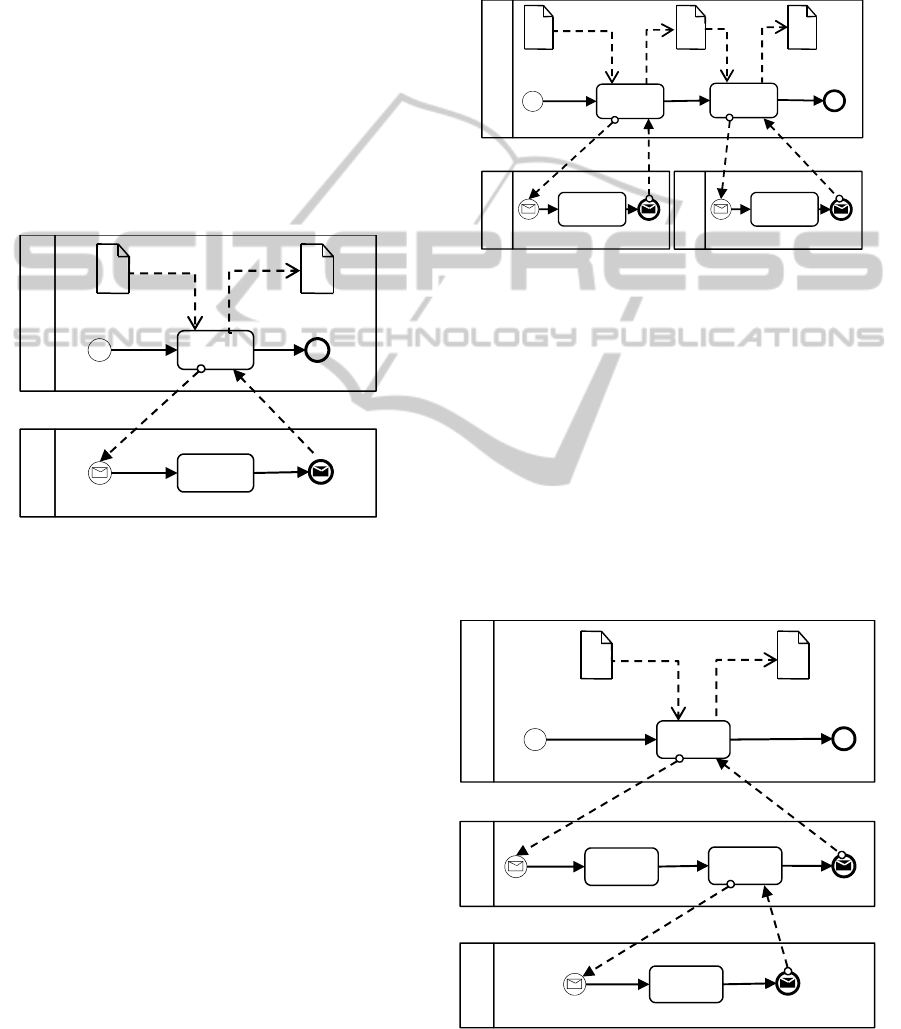
Figure 2: Simple optimization pattern in BPMN.

A BPMN diagram with two pools representing two

participants, the optimization algorithm and the

solver respectively, can be used to model the simple

optimization pattern, as shown in Figure 2. The

optimization algorithm is defined with a process

with three nodes: a start event, a task that

implements the optimization algorithm itself, and an

end event that are executed in sequence. The

optimization task (labeled as OA) gets the initial set

of designs to evaluate from a data object (DoE) and

produce the final Pareto front in a second data object

(Pareto). The solver is implemented also by a three

nodes process: a message triggered start event, a task

that implements the solver itself and an end event

that generates a message. When the OA task

generates a message with the design to be evaluated

as payload, an instance of the second process is

started. The solver (S) evaluates the design and

generates a message with the corresponding metrics

as payload, which is sent to the optimization task

(OA) through the conversation defined between the

two participants. Multiple instances of the solver can

be run in parallel, each one of them started when

triggered by the message from the optimization

task.

A sequential optimization pattern can be

represented by adding a second optimization

algorithm task in the first process, as shown in

Figure 3. The first optimization task (labeled as

Figure 3: Sequential optimization pattern in BPMN.

) gets the initial set of designs to evaluate from a

data object (DoE), performs the evaluation using the

first solver (S), producing as output a set of designs

which are assigned to a data object (Best designs).

The second optimization algorithm (OA

) uses this

data object as the initial population for the second

optimization loop, which in turn produces the final

Pareto front in a third data object (Pareto) by

repeatedly evaluating designs by using the second

solver (S’). Note that multiple instances of the solver

can be run in parallel for each optimization cycle.

Figure 4 presents the nested optimization

pattern represented in BPMN. The two optimization

Figure 4: Nested optimization pattern in BPMN.

Pareto

OAS

DoE

DoE Pareto

OAS

Bestdesigns

NOAS'

NOA

ParetoDoE

TowardsaStandardApproachforOptimizationinScienceandEngineering

173

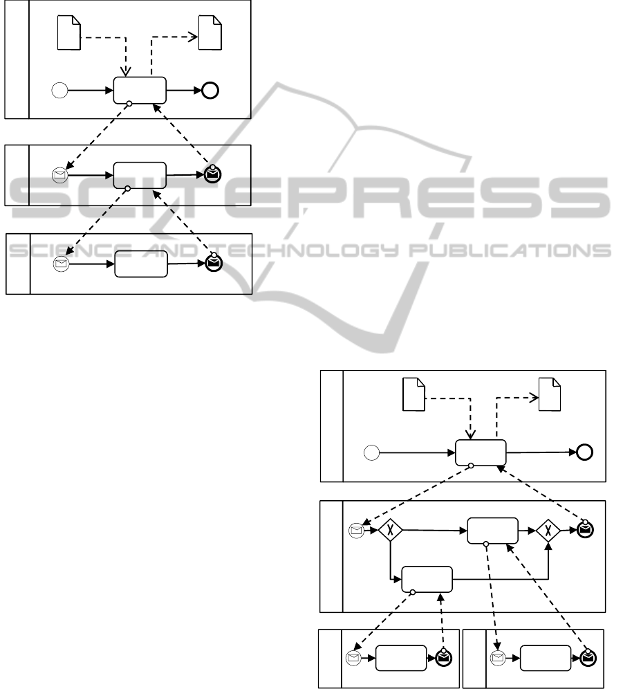
loops are implemented in different processes. The

first process (OA) implements the outer optimization

loop in the same terms as the loop in the simple

optimization pattern, sending designs for evaluation

to the inner optimization loop (NOA). An instance

of this process is started for every message

Figure 5: Robust optimization pattern in BPMN.

received, meaning that multiple inner optimizations

can be evaluated concurrently. The internal

optimization executes a solver (S), and based on

their output and the design sent from the external

optimizer, performs a local optimization by using

the nested algorithm (NOA). The nested algorithm

evaluates designs by using the second solver defined

in the third process (S’). Note that evaluations of the

this process can also be run concurrently.

Figure 5 shows the robust optimization pattern

in BPMN, which represents a very usual pattern in

industrial design. There is an optimization algorithm

task (OA) which sends through messages the designs

for evaluation to the second process. One instance of

this process is started for each design that is

received.

The robust sampling task (RS) generates a

number of messages for each design received from

the top level, which are in turn sent as messages to

the third process for evaluation by using the solver

(S). Note that if the first process generates n

messages for concurrent evaluation, n process for

robust sampling will be started concurrently, and if

the RS processes send each one m messages for

concurrent evaluation, a total of solver

instances could eventually be run concurrently.

The mixed robust optimization pattern in

BPMN is shown in Figure 6. In this patter there is an

external optimization loop which send designs for

evaluation to the robust sampling process as in the

previous pattern (see Figure 5). This process

performs evaluations by using the real solver (S) or a

synthetic model of it (RSM) depending on a

probabilistic distribution, a decision that is

represented with the decision exclusive gateway

node in the second process.

4.4 Efficiency Considerations

The previous section has shown that BPMN can be

used to represent the most widely used patterns in

optimization. However, in order to use it effectively

in a real environment, execution efficiency has also

to be considered. Many aspects in the BPMN

specification can introduce execution difficulties for

optimization workflows. Nevertheless, the BPMN

extension mechanisms allows defining new elements

to effectively handle them. Since it is not possible to

describe all situations that have been considered, this

section presents a representative example that

shows how a typical problem with efficiency can be

handled with appropriate extensions. The next

section will present experimental results by using the

extension proposed.

As shown before, optimization patterns are

Figure 6: Mixed robust optimization pattern in BPMN.

heavily based on asynchronous communication. This

puts a strong pressure on the messaging system,

Pareto

OARS

DoE

RSM

ParetoDoE

VRS

ICSOFT2013-8thInternationalJointConferenceonSoftwareTechnologies

174

since optimization processes typically run for a long

time, with days or weeks being a common duration,

involving also a large number of task evaluations.

Hundreds of thousands of messages could be

exchanged in a single run. In a typical robust

optimization problem (as show in Figure 1.d), if the

optimization algorithm (OA) sends n designs for

evaluations, n concurrent instances of the robust

sampling (RS) process will be started (



,1 

). If each one of these instances send m randomly

perturbed designs for evaluation, then nm

concurrent solver (S) instances will be started





,1,1). Messages sent back

from the S

instance need to be addressed to the

correct RS

instance, and messages sent back from

the RS instances has be addressed to the correct OA

instance.

BPMN uses a correlation mechanism to

associate messages to particular instances involved

in a conversation (OMG, 2011). Exchanged

messages are correlated through the so-called

correlation keys, which are defined as a set of

name-value pairs. In simplified terms, when the first

message in a conversation is received, the receiver

process stores the correlation values for the key,

which must match in future interchange of

messages. In this way, messages can be routed to the

appropriate instance responsible for receiving the

message. For the robust optimization pattern (see

Figure 5), two correlation keys are required, one to

correlate messages between OA and RO, and other

to correlate messages between RO and S. The first

key can be the design ID, while the second can be a

combination of the design ID and the sequence

number of the perturbed design.

Note that a process needs to keep information

about all keys that are used in order to eventually

match future messages. This implies an extra

memory requirement to store the keys and

additionally, extra processing time to perform the

matching process every time a new message is

received. These problems can be easily solved by

adding an extension element to indicate the time to

live (TTL) for messages, representing the number of

steps expected in a conversation that uses a

particular correlation key. As can be noted from the

selected pattern, single request-response means that

the key can be discarded as soon as an answer

message is received, removing the need to store the

keys for checking future matching since there will

never be other answer. The following XML code

shows an example of the use of the extension TTL

added to the conversation element of BPMN:

<optimization:TTL value="1"/>

</extensionElements>

. . .

Of course, the TTL extension can be used at

workflow designer discretion, meaning that he or

she should include it only when it is clear from the

communication pattern.

5 IMPLEMENTATION

In order to demonstrate practically the effect of

efficiency enhancement by using the extension

mechanism, this section presents the experimental

results of the TTL extension presented in previous

section. The pattern considered is the robust

optimization flow, which has been presented in

Figure 5. In order to make more evident the effect

of the TTL enhancement, an unlimited value of 

as perturbation for robust optimization was selected.

Figure 7 presents the results of the execution in

Figure 7: Memory usage for a robust optimization

execution with TTL (continuous line) and without TTL

(dotted line).

terms of memory consumption. Memory usage

without TTL is plotted with a dotted line, while

memory usage with the TTL extension is plotted

with a continuous line. As it can be appreciated,

memory requested from the heap grows

continuously due to the need to store the correlation

keys when TTL is not used. The problem arises

because the RS process cannot discard a key, even

if its associated message has been received, since the

standard specifies that other messages with the same

key can eventually arrive. The optimizer workflow

designer knows by sure that this will never happen,

but there is no way in which he or she can specify it.

The continuous line plot in Figure 7 shows that with

TowardsaStandardApproachforOptimizationinScienceandEngineering

175

the TTL extension, the use of memory is stable,

updated only at regular intervals by the execution of

the garbage collector. This happens because

correlation keys are disposed as soon as a message

that matches the corresponding key is received,

releasing the memory that was occupied by the key.

A similar effect can be appreciated with the

processing time. Figure 8 presents the results of the

delay in the execution of the solver process over

time. Delay without TTL is plotted with a dotted

line, while delay with the TTL extension is plotted

Figure 8: Delay to start the solver with the TTL extension

(continuous line) and without it (dotted line).

with a continuous line. With the no-TLL approach,

every time a message arrives, the matching process

has to consider all correlation keys, including the

values that have successfully matched a message

before. The TTL approach instead presents no delay,

since correlation keys are removed as soon as the

message has been processed, with no need to include

them in the matching process.

6 CONCLUSIONS

Optimization workflows have been used

successfully over many years; however, the

currently available tools used for their definition and

execution are not based on standard technologies. A

large number of different graphic and execution

formats are currently in use, and there is no clear

signs of convergence until to date. This paper has

proposed the use of BPMN 2.0, a well-defined

standard from the area of business processes, as a

formal representation for both the abstract and the

execution model for optimization workflows. In

particular, it was shown that BPMN 2.0 can support

the most widely used optimization patterns required

today in industry. An implementation example that

illustrates the use of BPMN 2.0 extensions to solve a

representative execution efficiency problem has also

been presented.

It is expected that the use of a standard for

optimization workflows will facilitate the

collaboration between scientists and industrial

designers, enhance the interaction between different

engineering and scientific fields, providing also a

common vocabulary in scientific and engineering

publications.

REFERENCES

Abramson D., Bethwaite B., Enticott C., Garic S., Peachey

T., 2011. Parameter Exploration in Science and

Engineering Using Many-Task Computing. In IEEE

Transactions on Parallel and Distributed Systems, vol.

22, no. 6, pp. 960-973. IEEE.

Abramson D., Bethwaite B., Enticott C., Garic S., Peachey

T., Michailova A., Amirriazi S., Chitters R., 2009.

Robust Workflows for Science and Engineering. In

Proceedings of the 2nd Workshop on Many-Task

Computing on Grids and SupercomputersMTAGS’09.

ACM.

Abdelahad C., Riesco D., Comin C., Carrara A., Kavka,

C., 2012. Data Transformations using QVT between

Industrial Workflows and Business Models in

BPMN2. In The Seventh International Conference on

Software Engineering Advances ICSEA 2012. IARIA.

Berthold, M. et al, 2008, KNIME: The Konstanz

Information Miner. In Data Analysis, Machine

Learning and Applications, ed. Bock H, Gaul W.,

Vichi, M., pp. 319-326, Springer.

Bertsimas D., Brown D., Caramanis C., 2010, Theory and

Applications of Robust Optimization. SIAM Review,

vol. 53 no. 3, pp. 464-501. SIAM.

Branke, J., Deb, K., Miettinen, K., Slowinski, R., 2008.

Multiobjective Optimization, Interactive and

Evolutionary Approaches. In Lecture Notes in

Computer Science, vol. 5252, Springer.

ESTECO SpA, 2012, modeFRONTIER applications

across industrial sectors involving advanced

CAD/CAE packages, (online) Available at:

<http://www.esteco.com/home/mode_frontier/by_indu

stry>, (retrieved: 14 February 2013)

Lin C., Lu S., Fei X. at al, 2009, Reference Architecture

for Scientific Workflow Management Systems and the

VIEW SOA Solution. In IEEE Transactions on

Service Computing, vol. 2, no. 1, IEEE.

Ludascher B., Altintas I., Bowers S. et al., 2009. Scientific

Process Automation and Workflow Management. In

Scientific Data Management: Challenges, Technology,

and Deployment, edited by Shoshani A., Rotem D.

Chapman and Hall.

Missier P., Soiland-Reyes S., Owen S., Tan W., Nenadic

A., Dunlop I., Williams A., Oinn T., Goble C., 2010,

Taverna, Reloaded. In Lecture Notes in Computer

ICSOFT2013-8thInternationalJointConferenceonSoftwareTechnologies

176

Science, vol. 6187, pp. 471-481, Springer.

OMG (Object Management Group), 2011, Business

Process Model and Notation. (online) Available at:

<http://www.omg.org/spec/BPMN/2.0> (Accessed 14

February 2012).

Sonntag M., Karastoyanova D., Deelman E. , 2010.

Bridging The Gap Between Business And Scientific

Workflows. In Proceedings of the 6th IEEE

International Conference on e-Science. IEEE

Computer Society.

Taylor I., Shields M., Wang I., Harrison A., 2007, The

Triana workflow environment: architecture and

applications. In Workflows for e-Science: Scientific

Workflows for Grids, I. Taylor et al., Eds. Springer.

Voutchkov I., Keane A., 2010, Multi-objective

Optimization Using Surrogates. In Computational

Intelligence in Optimization, ed. Tenne Y., Goh C., pp.

155-175, Springer

TowardsaStandardApproachforOptimizationinScienceandEngineering

177