Data Location Optimization Method to Improve Tiered
Storage Performance
Shinichi Hayashi
1
and Norihisa Komoda
2
1
Yokohama Research Laboratory, Hitachi, Ltd., Kanagawa, Japan
2
Graduate School of Information Science and Technologies, Osaka University, Osaka, Japan
Keywords: Data Location Optimization, Tired Storage, Dynamic Tier Control, I/O Performance, SSD.
Abstract: We propose a new method for tiered storage and evaluate the characteristics of the method. In this method,
a fast tier is divided into two areas, and the data in each area is managed on the basis of two input/output
(I/O) measurement periods. When I/Os to these areas increase, the proposed method allocates frequently
accessed areas to a higher tier in advance, therefore, improving the total system I/O performance. When
frequently accessed areas rarely move, the proposed method is the most effective and improves the total
system I/O performance by up to 30.4%.
1 INTRODUCTION
With recent improvements in information
technology, the amount of data retained by
companies has increased exponentially. The capacity
of hard disk drives (HDDs) has continued to
increase; however, the performance of these devices
has not improved significantly. Therefore, HDDs
can potentially become bottlenecks. Solid state
drives (SSDs), which are much faster than HDDs,
are currently attracting attention. When HDDs are
bottlenecks, replacing HDDs with SSDs could
potentially increase performance. However, SSDs
are generally more expensive and have less storage
capacity. Therefore, budget and capacity constraints
limit a company’s ability to replace all HDDs with
SSDs.
In General, input and output (I/O) activities have
a locality, and the number of I/Os for each storage
area is different. Therefore, if frequently accessed
areas are stored on a SSD and rarely accessed areas
are stored on a HDD, I/O performance will increase
and system cost will be reduced. A frequently
accessed area is denoted as a hot area and a rarely
accessed area is denoted as a cold area.
We define media in different levels of
performance as storage tiers and define storage that
leverages several tiers as a tiered storage. Several
reports have investigated tiered storage, and several
companies provide tiered storage (Hitachi, 2012)
(Schmidt et al., 2012) (EMC, 2012) (Hewlett-
Packard, 2012). Tiered storage moves data to an
appropriate tier on the basis of the number of I/Os,
as described above. In this paper, this function is
denoted as “Dynamic Tier Control.” In Dynamic
Tier Control, the storage measures the number of
I/Os for each area for a certain period, which is
denoted as the “I/O measurement period.” On the
basis of this measurement, the stored data is moved
to an appropriate tier. I/O measurement period also
indicates the frequency of data movement between
tiers.
To increase system performance, hot areas
should be allocated to a faster tier. This could be
accomplished by shortening the I/O measurement
period, because areas that become hotter are moved
to a faster tier immediately. However, this would
result in frequent data movements between tiers and
would have a negative impact on regular I/O
between servers and storage. On the other hand, if
the I/O measurement period was longer, data
movements between tiers would be reduced.
However, in this case, cold areas would remain
allocated to the faster tier. As a result, system I/O
performance would decrease.
In this paper, to address the above problem, we
propose a new fast tier allocation method on the
basis of short and long I/O measurement periods.
Since the effects of our proposed method will differ
depending on application I/O characteristics, I/O
measurement periods, and the rates of capacity of
112
Hayashi S. and Komoda N..
Data Location Optimization Method to Improve Tiered Storage Performance.
DOI: 10.5220/0004415901120119
In Proceedings of the 15th International Conference on Enterprise Information Systems (ICEIS-2013), pages 112-119
ISBN: 978-989-8565-59-4
Copyright
c
 2013 SCITEPRESS (Science and Technology Publications, Lda.)

the fast tier, we use a simulation to evaluate our
proposal.
2 EXISTING METHOD
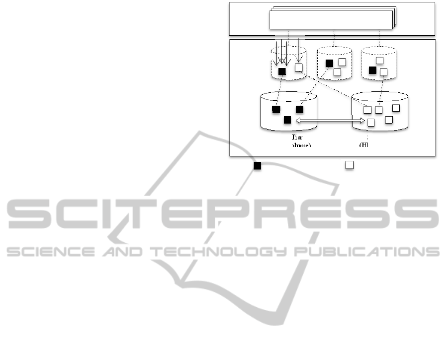
2.1 Dynamic Tier Control
In this section, we describe Dynamic Tier Control,
represented schematically in Figure 1. Applications
running on a server send I/O commands to virtual
volumes. The virtual volumes consist of small areas
called pages. Performance varies depending on
different types of volume. For example, the fast tier
is a SSD volume and the slow tier is a HDD volume
in Figure 1. An area of HDD or SSD volume is
allocated to each page. To determine the tier to
which pages are allocated, the storage measures the
number of I/Os to each page over a specific period
of time, ranks pages in order of the number of I/Os
for all pages in the storage, and allocates hot pages
to the fast tier. As a result, the storage moves data to
the appropriate tier.
To improve performance, the hottest pages need
to be allocated to the fastest tier for all volumes
within the entire storage system. We define the rate
of the number of I/Os for the fast tier to the total
I/Os as a fast tier I/O rate. To improve performance
of the entire storage system, the fast tier I/O rate has
to be high.
2.2 Problems with the Existing Method
Typically, it is considered that shortening the I/O
measurement period will increase the fast tier I/O
rate under Dynamic Tier Control. When the number
of I/Os to a page changes and the page becomes hot,
the storage can allocate a fast tier to the page
immediately using shorter I/O measurement periods.
For example, when the I/O measurement time is 24
hours, pages that have become hot during this period
continue to be allocated to a slow tier for the
duration of the period. When the I/O measurement
time is one hour, the storage system allocates pages
that have become hot to a fast tier after one hour.
However, when the I/O measurement period is
shorter, the storage has to move data between tiers
more frequently. Because SSDs are more expensive
than HDDs, to improve cost performance, all SSD
areas are allocated to pages and used. Therefore,
when hot areas change, the storage has to move the
coldest pages residing on the fast tier to the slow
tier. Pages allocated to the slow tier that become hot
Figure 1: Overview of the Existing Method.
are reallocated to the fast tier. Consequently, the
number of I/Os between tiers will increase, which
will result in a negative impact on regular I/O
between servers and the storage. Therefore,
decreasing the number of data movements between
tiers is important.
Increasing the I/O measurement period would
reduce migration between tiers. However, hot areas
that become cold would remain on the slow tier and
cold areas that become hot would remain on the fast
tier, and overall storage performance would be lower.
2.3 Related Research
In this section, we describe previous research related
to improving existing Dynamic Tier Control. Zhang
et al. (2010) have described an adaptive and
automated lookahead data migration method to
allocate hot areas to the fast tier on the basis of I/O
history before initiating a batch process. Typically,
Dynamic Tier Control allocates hot pages to the fast
tier after a batch process starts. Allocating hot pages
to a fast tier prior for the initiation of a batch process
improves performance. In order to apply this
method, the status of pages designated as hot areas
cannot change during the batch process. It would be
impossible to anticipate which pages would be hot if
the page status changed during processing.
3 PROPOSED METHOD
In this section, we explore the reason why the
problem, as described above, occurs if a single I/O
measurement period is used. We propose a new
method to allocate hot pages to a fast tier using two
Fast Tier
(SSD Volume)
Slow Tier
(HDD Volume)
Virtual
Volume
Applications
Frequently Accessed Page Occasionally Accessed Page
Data
Movement
between Tiers
I/O
Server
Storage
DataLocationOptimizationMethodtoImproveTieredStoragePerformance
113

different I/O measurement periods, a long period
and a short period.
To increase the fast tier I/O rate without
shortening the I/O measurement period, we consider
allocating pages that are expected to be hot to the
fast tier. Even if pages that have been hot for a long
time become cold, it is anticipated that this change is
temporary and that the pages will become hot again.
Therefore, areas that are hot for a short time as well
as areas that are hot for a long time should be
allocated to the fast tier. Under the existing method,
when area conditions change, the probability of
allocating areas that have already become hot to a
fast tier is low. These hot areas remain allocated to a
low tier for the duration of the I/O measurement
period; however, the proposed method increases the
probability that the areas that become hot are already
allocated to a fast tier. This improves overall system
I/O performance.
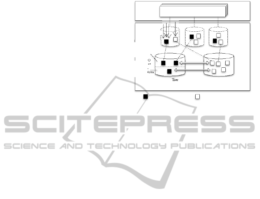
The proposed method is illustrated in Figure 2.
The fast tier is divided into two areas. A long I/O
measurement period is applied to the first area and a
short I/O measurement period is applied to the
second area. Here, the long I/O measurement period
is 24 hours and the short I/O measurement period is
one hour. At the end of each I/O measurement
period, the storage runs a process to determine
which pages should be allocated to the fast tier. It
runs the process every 24 hours to allocate pages to
the long I/O measurement period applied area on the
basis of the number of I/Os for last 24 hours. After
that, it allocates pages every one hour to the short
I/O measurement period applied area except the
pages that have been allocated to the long I/O
measurement period applied area on the basis of the
number of I/Os for last 1 hour.
4 EVALUATIONS
To evaluate the proposed method, we assess system
I/O performance improvements and the reduced
amount of data movements between tiers.
4.1 Simulation Condition
To validate the practical application and
effectiveness of the proposed method, we simulate
I/Os from a server to storage and data migrations
between tiers on the basis of I/O log data (Hewlett-
Packard, 2012) captured from a real environment.
There are many I/O patterns in a real
Figure 2: Overview of the Proposed Method.
environment. For example, I/Os can be concentrated
or distributed, and hot areas may move or not move.
Therefore, we generate 31 patterns to simulate I/Os
from the server to the storage on the basis of this I/O
log data. We define condition A as being equal to
the original I/O log data. Peak I/Os in the log data
occur between 3:00 to 6:00 a.m., and the number of
I/Os is large at this time. The number of I/Os for
other time periods is smaller than the peak time and
stable.
Table 1 shows the I/O pattern conditions
generated from one month of I/O log data. The
upper row of each cell shows the condition and the
lower row of each cell shows the number of I/Os per
second from application to storage. Each condition
is a repetition of a three hour period of I/O log data
from each day of the one month period. The time
frames for each condition are as follows: Condition
B is 12:00 to 3:00 a.m.; condition C is 10:00 p.m. to
1:00 a.m.; condition D is 2:00 to 5:00 p.m.;
condition E is 12:00 a.m. to 3:00 p.m.; condition F is
11:00 a.m. to 2:00 p.m.; and condition G is 10:00
a.m. to 1:00 p.m. The I/O locality for each condition
is different, which is representative of the workload
in a real environment. Therefore, we create six I/O
patterns; I/O for condition B is the most
concentrated, and I/O for condition G is the least
concentrated on the basis of locality these conditions
are selected. Figure 3 shows the I/O distribution for
these conditions. The horizontal axis shows the
accessed page rate in the total pages, and the vertical
axis shows an accumulative total I/O rate. For
example, 63% of I/Os occur on 10% of the storage
capacity, 84% of I/Os occur on 20% of the capacity,
and 95% of I/Os occur on 30% of the capacity for
condition B.
Fast Tier Slow Tier
Virtual
Volume
Applications
Frequently Accessed Page
Occasionally Accessed Page
Data
Movement
between Tiers
I/
O
Server
Storage
Short I/O
Measurement Period
Applied Area
Long I/O
Measurement
Period
Applied Area
ICEIS2013-15thInternationalConferenceonEnterpriseInformationSystems
114

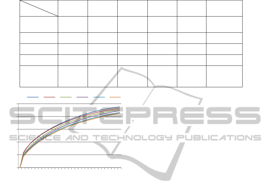
Table 1: Simulation Condition.
Condition B
(High
Locality)
Condition C Condition D Condition E Condition F
Condition G
(Low Locality)
Condition 1h
(Frequent
Movement)
B-1 h
78 IOPS
C-1 h
64 IOPS
D-1 h
76 IOPS
E-1 h
73 IOPS
F-1 h
80 IOPS
G-1 h
85 IOPS
Condition 3h
B-3 h
78 IOPS
C-3 h
64 IOPS
D-3 h
76 IOPS
E-3 h
73 IOPS
F-3 h
80 IOPS
G-3 h
85 IOPS
Condition 6h
B-6 h
78 IOPS
C-6 h
64 IOPS
D-6 h
76 IOPS
E-6 h
73 IOPS
F-6 h
80 IOPS
G-6 h
85 IOPS
Condition 12h
B-12 h
78 IOPS
C-12 h
64 IOPS
D-12 h
76 IOPS
E-12 h
73 IOPS
F-12 h
80 IOPS
G-12 h
85 IOPS
Condition
“Not Move”
(Occasional
Movement)
B-Not
Move
78 IOPS
C-Not Move
64 IOPS
D-Not Move
76 IOPS
E-Not Move
73 IOPS
F-Not Move
80 IOPS
G-Not Move
85 IOPS
Figure 3: I/O Distribution.
Moreover, we assume that there are two unique
I/O usage cases: (1) only one application continues
to run and accessed areas do not move and (2)
running applications change by schedule and
accessed areas move. Therefore, we create another
condition that considers the movement of accessed
areas. Condition 1 h is for accessed areas moving
every hour; condition 3 h is for accessed areas
moving every three hours; condition 6 h is for
accessed areas moving every six hours; condition
12 h is for accessed areas moving every 12 hours;
and condition Not Move is for accessed areas that do
not move. We define this cycle as an I/O movement
cycle. Accessed areas move every I/O movement
cycle, and the areas move to the same areas on the
next day. The combinations of conditions B to G and
conditions 1 h to 24 h result in 30 total conditions
ranging from B-1 h to G-Not Move.
Page size is generally between 1 MB and 1 GB
when applying Dynamic Tier Control. Page size is
10 MB in this simulation, and the number of pages is
8,679. We define the rate of fast tier capacity in the
total capacity as the fast tier capacity rate. The fast
tier capacity rate increases from 5% to 30% in
increments of 5% in this simulation. Since
application to storage I/Os have locality and fast tier
media is generally expensive, fast tier capacity rate
is 5% to 30% for general use to increase cost
performance.
The I/O measurement periods are 1, 3, 6, 12, and
24 hours for the existing method. We define the fast
tier capacity rate by applying the short I/O
measurement period as a short period movement
capacity rate. The short period movement capacity
rate is increased by 10% from 10% up to 90% in the
proposed method. The short I/O measurement period
is 1 hour and the long I/O measurement period is 24
hours because an I/O measurement period is
generally 1 to 24 hours.
4.2 Evaluation Method
We define the number of I/Os that the storage can
process per minute as storage I/O performance. The
storage I/O performance is the sum of the number of
application to storage I/Os and the number of data
movement I/Os between tiers. The total system I/O
performance is the storage I/O performance minus
data movements between tiers. The total system I/O
performance (


,

[IOPS]) is calculated
from formula (1). This formula is based on previous
research (Matsuzawa et al., 2012).  [%] is the fast
tier capacity rate;  [hours] is the I/O measurement
time; 

,


[%] is the fast tier I/O rate; 

[IOPS] is I/O performance on the fast tier; 

[IOPS] is I/O performance on the low tier; and


,

[%] is the number of I/Os per second of
data movements between tiers.
0%
20%
40%
60%
80%
100%
0% 2% 4% 6% 8%
10% 12% 14% 16% 18% 20% 22% 24% 26% 28% 30%
I/ORate[%]
CapacityRate[%]
A B C D E F
Condition B C D E F G
DataLocationOptimizationMethodtoImproveTieredStoragePerformance
115

Table 2: Parameters of Each Tier.
Media SSD HDD
Maximum I/O Performance Ratio 180 1
The total system I/O performance
( 

, 

,

, ) [IOPS]) is
calculated from formula (2) in the proposed method
where 

[hours] is the short I/O measurement
period; 

[hours] is the long I/O measurement
period;
C [%] is the short period movement capacity
rate; and 

, 

,

, [%] is the fast
tier I/O rate.
From the simulation results, we calculate the
total system I/O performance per hour and calculate
the monthly average total system I/O performance
under the existing method.
Table 2 shows the simulation parameters for
each tier. Based on previous research (Emaru et al.,
2011), the I/O performance of the fast tier is 180
times higher than that of the slow tier and the I/O
performance for each tier of random read, random
write, sequential read, and sequential write is 25%,
respectively, and the I/O size is 8 KB.
4.3 Results and Discussion of the
Experiment with Original I/O
Log Data
Figure 4 shows the total system I/O performance
improvement rates of the existing and the proposed
methods under condition A. The horizontal axis
shows the conditions; the short data movement
capacity rate for the proposed method and the I/O
measurement period for the existing method. The
vertical axis shows the total system I/O performance
improvement rate where the total system I/O
performance is 100% and the I/O measurement
period is 24 hours (normalized).
Figure 5 shows the amount of I/Os for the data
movements between tiers for the existing and
proposed methods under condition A. Similar to
Figure 4, the horizontal axis shows the conditions.
The vertical axis shows the rate of the number of
I/Os for movements between tiers to the total
Figure 4: Total System I/O Performance Improvement
Rate.
number of I/Os from application to storage.
In Figure 4, in the case that the fast tier capacity
rate is 5% and 10%, the total system I/O
performance is the highest when the I/O
measurement period is four hours in the existing
method. The I/O measurement period where the total
system I/O performance is the highest becomes
shorter as the fast tier capacity rate becomes higher.
The storage I/O performance is in the highest when
I/O measurement time is one hour, regardless of fast
tier capacity rate. However, the total system I/O
performance is lower when the I/O measurement
period is one hour due to the heavy data movements
between tiers. For example, when fast tier capacity
rate is 20%, the total system I/O performance
decreases by 17% due to the heavy data movements
between tiers.
In Figure 5, in the case of a one hour I/O
measurement period, the amount of data movements
between tiers is the largest when the fast tier
capacity rate is 20%. In the case of a fast tier
capacity rate being greater than 20%, many areas
can be allocated to the fast tier because there is less
data movement between tiers when hot areas are
moved.
Here, we discuss the proposed method’s
simulation results. In the case of a fast tier capacity
rate being 10% or more, the total system I/O
performance with the proposed method is the highest
and is better than the results for the existing method
when the short period movement capacity rate is



,


1



,




1


,



,
(1)


, 

,

,

1


, 

,

,



1

, 

,

,


,

,

,
(2)
90%
100%
110%
120%
130%
140%
150%
10% 20% 30% 40% 50% 60% 70% 80% 90%
1時間 2時間 4時間 6時間
12時間 24時間
Condition
5% 10% 15%
20% 25% 30%
Fast TierCapacityRate
ProposedMethod
Existing Method
S
y
stemTotalI
/
OPerfromanceIm
p
rovement
Rate[%](Normalized,Existing 24h=100%)
1h
2h
4h
6h
12h
24h
ShortPeriodMovementCapacityRate
13.8x
I/OMeasurement
ICEIS2013-15thInternationalConferenceonEnterpriseInformationSystems
116

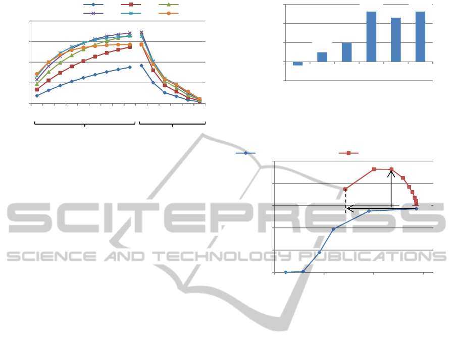
Figure 5: I/O Rate of Data Movements.
20% or 30%. In the case of the fast tier capacity rate
of 10% and a higher period capacity rate, the fast tier
I/O rate is higher; however, the total system I/O
performance is lower. This is because the amount of
data movement between tiers increases even though
the fast tier I/O rate increases.
In the proposed method, when the short period
movement capacity rate increases, the amount of
data movement between tiers increases. In the case
of a short period capacity rate increase, the amount
of data movement between tiers increases in a short
time.
Figure 6 shows the total system I/O performance
improvement rate for each fast tier capacity rate
under the proposed method. The horizontal axis
shows the fast tier capacity rate. When the fast tier
capacity rate is 30%, the total system I/O
performance rate is the highest, showing an increase
of 13.8%.
In the case of a fast tier capacity rate of 5%, the
total system I/O performance decreases by 1.0%
with the proposed method. This is because the top
5% of frequently accessed areas move very
infrequently. Therefore, when the proposed method
is applied, the fast tier I/O rate and the total system
I/O performance are not relatively changed
compared to the existing method.
Figure 7 shows the relationship between the total
system I/O performance (Figure 4) and the amount
of data movement between tiers (Figure 5).The
vertical axis shows the total system I/O performance
improvement rate. The horizontal axis shows the
amount of data movement between tiers. In the case
of a fast tier capacity rate of 30% under the existing
method, when the I/O measurement period is one
hour, the total system I/O performance improvement
rate is 129%, and the amount of data movement
between tiers is 14.3%. In the case of a short period
capacity rate of 10% under the proposed method, the
Figure 6: Total System I/O Performance Improvement
Rate.
Figure 7: Relationship between Total System Performance
and the Amount of Data Movements between Tiers.
total system I/O performance improvement rate is
137% and the amount of data movement between
tiers is 7.15%. The total system I/O performance
does not decrease, and the amount of data movement
between tiers decreases by 50.0%. From these
results, it can be seen that the proposed method
improves total system I/O performance without
increasing data movement between tiers.
4.4 Results and Discussion of the
Experiment with Generated I/O
Log Data
In this section, we discuss the results of the
simulation of conditions B-1 h to G-Not Move.
Figure 8 shows the storage I/O performance
improvement rate under the proposed method. The
horizontal axis shows the I/O movement cycle for
each condition. The vertical axis shows the storage
I/O performance improvement rate.
The higher the fast tier capacity rate is, the higher
the storage I/O performance improvement rate is. In
the case of a high fast tier capacity rate (e.g., 30%)
and more concentrated I/Os condition (e.g.,
0%
5%
10%
15%
20%
10% 20% 30% 40% 50% 60% 70% 80% 90%
1時間 2時間 4時間 6時間
12時間 24時間
I/ORateofDataMovementsbetween
Tiers[%](Normalized)
Condition
5% 10% 15%
20% 25% 30%
FastTier CapacityRate
ProposedMethod
ExistingMethod
1h
2h
4h
6h
12h
24h
ShortPeriodMovementCapacityRate I/OMeasurement
Period
‐1,0%
2,5%
4,9%
13,5%
11,5%
13,8%
‐5,0%
0,0%
5,0%
10,0%
15,0%
5% 10% 15% 20% 25% 30%
SystemTotalI/O
PerfromanceImprovement
Rate[%](Normalized)
FastTierCapacityRate[%]
100%
110%
120%
130%
140%
150%
0% 5% 10% 15%
SystemTotalI/OPerformanceRate[%]
(Normalized)
RateoftheAmountofDataMovements
betweenTiers[%]
従来手法 高速階層率30% 提案手法 高速階層率30%
24h
12h
6h
4h
2h
1h
10%
20%
30%
40%
50%
60%
70%
80%
90%
ExisgingMethod
(I/OMeasurementPeriod)
ProposedMethod
(ShortPeriod
Movoement
CapacityRate)
ExisgingFastTier=30%
ProposedFastTier=30%
−50.0%
+13.8%
DataLocationOptimizationMethodtoImproveTieredStoragePerformance
117

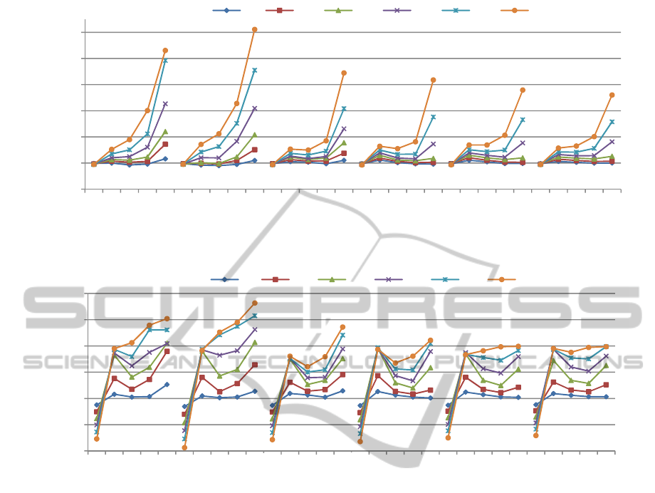
Figure 8: Storage I/O Performance Improvement Rate with Generated I/O Log Data.
Figure 9: Total System I/O Performance Improvement Rate with Generated I/O Log Data.
condition B or C), the storage I/O performance
improvement rate is high. However, in the case of a
low fast tier capacity rate (e.g., 5%), the storage I/O
performance improvement rate is equal to the
existing method regardless of I/O locality. This is
because the top 5% of frequently accessed areas is
typically file system management areas which rarely
move.
When the I/O movement cycle is longer, the
storage I/O performance improvement rate is higher.
When the I/O movement cycle is shorter, allocating
the fast tier with a shorter I/O measurement time is
less effective because hot areas move quickly and
there is no access to areas allocated to the fast tier.
From the above results and discussion, it is
evident that the storage I/O performance
improvement rate under the proposed method is
more effective when the fast tier capacity rate is
higher and the I/O movement cycle is longer. When
the fast tier capacity rate is low or the I/O movement
cycle is short, the storage I/O performance
improvement rate is the same as the existing method.
Figure 9 shows the total system I/O performance
improvement rate under the proposed method. The
horizontal axis shows the I/O movement cycle for
each condition. The vertical axis shows the total
system I/O performance improvement rate from the
best case under the existing method.
The higher the fast tier capacity rate is, the
higher the total system I/O performance
improvement rate is. In the case of a one hour I/O
movement cycle, the total system I/O performance
improvement rate under the proposed method is
lower than the existing method because the existing
method experiences less data movement between
tiers when the I/O measurement is 24 hours. In the
case of the condition B-Not Move, the total system
performance improvement rate is 136%.
From the above discussion, it is evident that the
total system I/O performance improvement rate
under the proposed method is the highest for all
conditions except when the I/O movement cycle is
one hour, the I/O movement cycle of one hour
existing method.
90%
100%
110%
120%
130%
140%
150%
1 3 6 12 24 1 3 6 12 24 1 3 6 12 24 1 3 6 12 24 1 3 6 12 24 1 3 6 12 24
StorageI/OPerformance
ImprovementRate[%](Normalized,
ExistingMethod=100%)
I/OMovementCycle[hours]
5% 10% 15% 20% 25% 30%
Condition B
Condition C
Condition D
Condition E
Condition F Condition G
FastTierCapacityRate
Move
Not
Move
Not
Move
Not
Move
Not
Move
Not
Move
Not
80%
90%
100%
110%
120%
130%
140%
1 3 6 12 24 1 3 6 12 24 1 3 6 12 24 1 3 6 12 24 1 3 6 12 24 1 3 6 12 24
SystemTotalI/OPerformance
ImprovementRate[%](Normalized,
ExistingMethod=100%)
I/OMovementCycle[hours]
5% 10% 15% 20% 25% 30%
ConditionB
FastTierCapacityRate
ConditionD
ConditionE
ConditionF
ConditionG
ConditionC
Move
Not
Move
Not
Move
Not
Move
Not
Move
Not
Move
Not
ICEIS2013-15thInternationalConferenceonEnterpriseInformationSystems
118

5 CONCLUSIONS
To increase total system I/O performance and
improve the amount data movement between fast
and slow tiers, we proposed a higher tier allocation
method on the basis of two I/O measurement periods
for a higher tier divided into two areas. Under the
proposed method, the total system I/O performance
rate is the highest and increases by up to 13.8%, and
the amount of data movement between tiers
decreases by up to 50.0%. The proposed method is
more effective than the existing method when the
fast tier capacity rate is high and frequently accessed
areas do not move.
REFERENCES
Hitachi Data Systems, Dynamic Tiering (online), available
from (http://www.hds.com/products/storage-software/
hitachi-dynamic-tiering.html) (accessed 10/9/2012)
Schmidt, G., Dufrasne, B., Jamsek, J., et al., IBM System
Storage DS8000 Easy Tier (online), available from
(http://www.redbooks.ibm.com/redpapers/pdfs/redp46
67.pdf) (accessed 7/28/2012)
EMC Corporation, Fully Automated Storage Tiering for
Virtual Pools (FAST VP) (online), available from
(http://www.emc.com/storage/symmetrix-vmax/fast.
htm) (accessed 7/28/2012)
Hewlett-Packard Development Company, HP 3PAR
Adaptive Optimization Software - Overview & Fea-
tures (online), available from (http://h18006.www.hp.
com/storage/software/3par/aos/index.html) (accessed
7/28/2012)
Zhang, G., Chiu, L., Liu, L., 2010. Adaptive Data
Migration in Multi-tiered Storage Based Cloud
Environment. Proceedings of the 3rd International
Conference on Cloud Computing, pp. 148-155
Zhang, G., Chiu, L., Dickey, C., et al., 2010. Automated
lookahead data migration in SSD-enabled multi-tiered
storage systems. Proceedings of the 26th Symposium
on Mass Storage Systems and Technologies, pp. 1-6
Hewlett-Packard Development Company, Cello99 Traces
(online), available from (https://tesla.hpl.hp.com/
opensource/) (accessed 7/28/2012)
Matsuzawa, K., Hayashi, S., Otani, T., 2012. Performance
Improvement by Application-aware Data Allocation
for Hierarchical Data Management. IPSJ SIG
Technical Report, No. 8, pp. 1-7
Emaru, H., Takai, Y., 2011. Performance Management for
the Dynamic Tiering Storage by Virtual Volume
Clustering. Journal of Information Processing, pp.
2234-2244
DataLocationOptimizationMethodtoImproveTieredStoragePerformance
119