Resource versus Space Competitions in a Plant Growth
Model
?
A. El Hamidi
Laboratoire LASIE, Université de La Rochelle, La Rochelle, France
Abstract. In this tutorial note, we present a spatiotemporal model for plant growth,
combining two different mechanisms of competition. The first mechanism con-
cerns the biomass growth via resources while the second concerns the space-
biomass expansion. The pure time mechanism is described by the standard un-
derlying Kolmogorov model for interacting populations. The spatial mechanism,
more adapted to plant growth, expresses the motility of each species and their
capability to exclude the others from its territory.
1 Introduction
The spatial and/or temporal behaviors of interacting species in ecological systems rep-
resent an important field in mathematical population ecology. In particular, competitive
dynamics of interacting species have been the subject of a sizeable literature. Various
mathematical models have been proposed to study problems of coexistence or exclu-
sion of competing species. Consider, for example, two substances (species, chemicals,
etc.) that are activating or inhibiting each other according to some law of reaction and
diffusing in a spatial domain by linear Fick’s law. The density of the two substances at
time t > 0 and place x ∈ Ω are denoted by u
1
(x, t) and u
2
(x, t) respectively, where Ω
is a bounded domain in R
2
.
The well-known competitive Lotka-Volterra-Gause type model is given by









∂u
1
∂t
− µ
1
∆u
1
= u
1
(α
1
− β
1
u
1
− γ
1
u
2
), t > 0, x ∈ Ω
∂u
2
∂t
− µ
2
∆u
2
= u
2
(α
2
− β
2
u
2
− γ
2
u
1
), t > 0, x ∈ Ω
(1)
where µ
i
is the the diffusion rate of u
i
, α
i
is the intrinsic growth rate, β
i
is the intra-
specific competition rate and γ
i
is the inter-specific competition rate.
Consider the case where all rates are positive constants and zero-flux boundary con-
ditions
∇u
i
(x, t) · n(x) = 0 on ∂Ω×]0, +∞[,
?
his work has been partially funded by CNRS (National Centre for Scientific Research) within
the framework of the "PEPS Rupture" call 2011
El Hamidi A..
Resource versus Space Competitions in a Plant Growth Model.
DOI: 10.5220/0004362200390045
In Proceedings of GEODIFF 2013 (GEODIFF-2013), pages 39-45
ISBN: 978-989-8565-49-5
Copyright
c
 2013 SCITEPRESS (Science and Technology Publications, Lda.)

where n(x) is the unit outward pointing normal at the point x to the boundary ∂Ω of
Ω. The initial conditions are
u
i
(x, 0) ≥ 0, for every x ∈ Ω.
It is well-known that stable attractors of (1) should be equilibrium solutions. This im-
plies that solutions of (1) become spatially homogeneous asymptotically, that is, stable
equilibrium solutions of the pure dynamical system associated to (1)



u
0
1
(t) = u
1
(α
1
− β
1
u
1
− γ
1
u
2
), t > 0,
u
0
2
(t) = u
2
(α
2
− β
2
u
2
− γ
2
u
1
), t > 0,
(2)
If the two species u
1
and u
2
are (ecologically) strongly competing, that is
β
1
γ
2
<
α
1
α
2
<
γ
1
β
2
,
the competitive exclusion principle between the u
1
and u
2
occurs [18, 17]. More pre-
cisely, any non-negative solution (u
1
, u
2
) converges to either (α
1
/β
1
, 0) or (0, α
2
/β
2
).
However, observations in natural fields show that strongly competing species can co-
exist. In [27], the authors show that this phenomenon can be assigned to the repulsive
effect between competing species. Indeed, they introduced cross-diffusion terms which
represent the environmental pressures due to the inter-specific interferences:









∂u
1
∂t
− ∆[(µ
1
+ au
2
)u
1
] = u
1
(α
1
− β
1
u
1
− γ
1
u
2
), t > 0, x ∈ Ω
∂u
2
∂t
− ∆[(µ
2
+ bu
1
)u
2
] = u
2
(α
2
− β
2
u
2
− γ
2
u
1
), t > 0, x ∈ Ω
(3)
where a, b stand for the cross-diffusion pressures and are nonnegative constants.
In what follows, we will present a model without cross-diffusions where the authors
[9] show that species with strong spatial competition can lead to their coexistence. In-
deed, the strong spatial competitions give rise to degenerate diffusions which guarantee
patterns formation and thus coexistence.
On the other hand, it is well known that System (2) has 4 equilibrium points:
(u
1
, v
1
) = (0, 0), (u
2
, v
2
) =

α
1
β
1
, 0

, (u
3
, v
3
) =

0,
α
2
β
2

,
(u
4
, v
4
) =

α
2
γ
1
− α
1
β
2
γ
1
γ
2
− β
1
β
2
,
α
1
γ
2
− α
2
β
1
γ
1
γ
2
− β
1
β
2

. Also, 4 situations of interest hold true,
in terms of the inter-specific competitions γ
1
and γ
2
:
(i)
γ
1
β
2
<
α
1
α
2
<
β
1
γ
2
(moderate competitions =⇒ coexistence of populations)
(ii)
β
1
γ
2
<
α
1
α
2
<
γ
1
β
2
(strong competitions =⇒ extinction of the initially disadvantaged
one)
(iii)
α
1
α
2
>
β
1
γ
2
and
α
1
α
2
>
γ
1
β
2
(strong vs weak competition =⇒ extinction of the
weak one)
40

0 0.2 0.4 0.6 0.8 1
0
0.2
0.4
0.6
0.8
1
0 0.2 0.4 0.6 0.8 1
0
0.2
0.4
0.6
0.8
1
Fig. 1. Left: Situation (i), right: Situation (ii).
0 0.2 0.4 0.6 0.8 1
0
0.2
0.4
0.6
0.8
1
0 0.2 0.4 0.6 0.8 1
0
0.2
0.4
0.6
0.8
1
Fig. 2. Left: Situation (iii), right: Situation (iv).
(iv)
α
1
α
2
<
β
1
γ
2
and
α
1
α
2
<
γ
1
β
2
(weak vs strong competition =⇒ extinction of the
weak one)
Notice that in all cases, the steady point (0, 0) is linearly unstable. Let us describe
the (linear) nature of the other steady states. In case (i), (u
2
, v
2
) and (u
3
, v
3
) are saddle
points and (u
4
, v
4
) is asymptotically stable. In case (ii), (u
2
, v
2
) and (u
3
, v
3
) are stable
and (u
4
, v
4
) is a saddle point.
On the other hand, we will see that the spatial competitions lead to similar situations,
linking the spatial and the time biomass competitions. In the best of our knowledge, this
fact is new and deserves more theoretical and numerical studies.
2 Spatial Competitions: Diffusion Degeneracy and Coexistence
In what follows, we present a simple pde’s model, without cross diffusions, that allows
coexistence and patterns formation, even for strongly competitive populations.
Consider the pde’s system









∂u
1
∂t
− div(µ
1
(u
2
)∇u
1
) = u
1
(α
1
− β
1
u
1
− γ
1
u
2
), t > 0, x ∈ Ω,
∂u
2
∂t
− div(µ
2
(u
1
)∇u
2
) = u
2
(α
2
− β
2
u
2
− γ
2
u
1
), t > 0, x ∈ Ω.
(4)
For a given parameter η
1
≥ 0, assume that
µ
1
(u
2
) > 0 if 0 ≤ u
2
≤ η
1
and µ
1
(u
2
) = 0 if u
2
> η
1
.
41

This system is degenerated because at least one diffusion term is not positive. In this
situation, species u
1
can not diffuse in locations where u
2
> η
1
and diffuses with the
rate µ
1
(u
2
) > 0 wherever 0 ≤ u
2
≤ η
1
. The parameter η
1
can be thus interpreted as
the ability of species u
2
to resist to the species u
1
intrusion; that is, if η
1
is small then
the exclusion ability of the species u
2
is large and vice versa. We expect that this kind
of degenerated diffusion can allow patterns formation without the presence of cross-
diffusion terms.
We will show that the role of η
1
in space competition is similar to that of γ
1
, in
resources competition. More precisely, for simplicity, consider the degenerated system









∂u
1
∂t
− div(µ(u
2
)∇u
1
) = u
1
(α
1
− β
1
u
1
− γ
1
u
2
), t > 0, x ∈ Ω
∂u
2
∂t
− div(µ(u
1
)∇u
2
) = u
2
(α
2
− β
2
u
2
− γ
2
u
1
), t > 0, x ∈ Ω
(5)
where
µ(s) > 0 if 0 ≤ s ≤ η and µ(s) = 0 if s > η.
The carrying capacity of the species u
1
and u
2
respectively K
1
:= α
1
/β
1
and K
2
:=
α
2
/β
2
, that is, the biomass u
1
satisfies the inequality 0 ≤ u
1
(x, t) ≤ K
1
for every
(x, t) ∈ Ω × [0, +∞[, provided that the initial condition u
1
(·, 0) satisfies the same
condition: 0 ≤ u
1
(x, 0) ≤ K
1
, for every x ∈ Ω. This fact is due to the positivity of the
diffusion µ and the Kolmogorov structure of the system (5). Similar properties can be
cited about the biomass u
2
.
In this special case, 4 situations of interest linking the spatial competition
– Infinite Spatial Competition: η = 0. In this situation, u
1
and u
2
can not coexist
in the same locations. In particular, u
1
and u
2
can not coexist in locations where
u
1
(x, 0) > 0 or u(x, 0) > 0.
– Strong Spatial Competition: 0 < η < min{K
1
, K
2
}. In this situation, u
1
and
u
2
can coexist but only in subdomains where the initial conditions satisfy: 0 ≤
u
1
(x, 0) ≤ η or 0 ≤ u
2
(x, 0) ≤ η.
– Weak Spatial Competition: η > max{K
1
, K
2
}. In this situation, the system
behaves as a non-degenerated one and the presence of diffusions does not impact
the linear stability of equilibrium points of (2). The exclusion principle takes place,
if at least one inter-specific competition rate is large (See Figure 3).
– Moderate Spatial Competition: min{K
1
, K
2
} < η < max{K
1
, K
2
}. In this
situation, the species with the greatest carrying capacity , that is, u
1
if K > K
2
or
u
2
if K
1
< K
2
, will be present alone in locations where its density exceeds η and
miscibility can occur elsewhere.
In the following, we present two simulations corresponding to the system (5) with
homogeneous Neumann boundary conditions on ∂Ω,
µ
1
(u
2
) ∇u
1
· n = µ
2
(u
1
) ∇u
2
· n = 0 on [0, +∞[×∂Ω.
The nonlinear diffusion coefficient is the truncation function
µ(s) = C exp

η
2
s
2
− η
2

, if 0 ≤ s < η and µ(s) = 0, if s ≥ η > 0.
42

We set C = exp(1) and hence 0 ≤ µ(s) ≤ 1. The parameters in the temporal dynamical
system (2) are such that the second species u
2
has a competitive advantage on the first
species, i.e unique stable equilibrium point

u
1
= 0, u
2
=
α
2
β
2
> 0

with
α
1
= 1, α
2
= 1.3, β
1
= 1.2, β
2
= 0.8, γ
1
= 3., γ
2
= 1.1.
We focus ourselves on two situations: the weak spatial competition and the weak
spatial competition cases. We test the competitive advantage of space exclusion that
corresponds to η  1 by comparing to the situation with quasi uniform diffusion η 
1.
The initial condition for the benchmark problem is a collection of well separated
sharp bell function
exp

−
dist((x, y), M
j
)
ν

,
that plays the role of initial "seeds of population density", centered on a set of points
M
j
- see Figure 3 and 4 at T = 0. We use a similar number of "seeds" for both species.
The numerical implementation is straightforward. We use a regular Cartesian grid
with a second order finite volume approximation in space and a second order Crank-
Nicolson implicit time stepping.
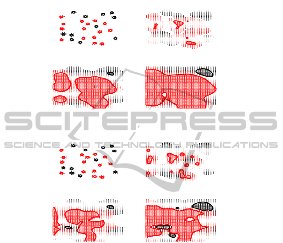
When we run the simulation, we observe at early time the diffusion process that
represents plant colonization. After some time, we start to see some interaction with
narrow fronts layers where both species compete. This boundary layer that separates
the species is more or less diffused depending on how small is the ν value.
In these figures we use the following convention: the space invaded by the first
species (respt. the second species) is marked by black label (respt. red label). The sim-
ulation exhibit then nice pattern formation for each species.
In the figures area where density is above 0.5 is indicated by circles ’o’, while the
area with lower concentration in the interval (0.1, 0.5) is indicated by dots ’.’. This helps
to visualize area where the first species is strongly dominant, i.e red circle zone, areas
where the second species diffuses every where black dot point area, and overlapping
zone where competition occurs.
As expected, for weak spatial competition, i.e η  1, the most competitive species
(0, α
2
/β
2
) wipe out the other one that goes to extinction, that is, weak competition has
no effect on the stability of uniform equilibrium points.
However, for strong spatial competition, i.e η  1, the stability of the uniform equilib-
rium point (0, α
2
/β
2
) can be modified by the strong spatial competition, which leads
sometimes to coexistence between strong competitive populations.
Eventually for infinite spatial competition, i.e η = 0, the less competitive species
will always survive, and perhaps get most of the field thanks to its initial fast space
invasion. In particular, the linear stability of equilibria is completely modified by this
infinite spatial competition.
43

T=0. T=1.2
T=2.4 T=3.6
Fig. 3. Two species system with weak spatial competition: η = 100, K
1
= 1/1.2 and K
2
=
1.3/0.8.
T=0. T=1.2
T=2.4 T=3.6
Fig. 4. Two species system with strong spatial competition η = 0.1, K
1
= 1/1.2 and K
2
=
1.3/0.8.
References
1. H. Amann, Nonhomogeneous linear and quadilinear elliptic and parabolic boundary value
problems. Function Spaces,Differential Operators and Nonlinear Analysis. H.J. Schmeisser,
H. Triebel (editors), Teubner, Stuttgart, Leipzig. (1993), 9-126.
2. R. Aris, The mathematical theory of diffusion and reaction in permeable catalysts. Vol. I:
The theory of the steady state. Oxford University Press. XVI, (1975).
3. F. Brauer, C. Castillo-Chavez, Mathematical Models in Population Biology and Epidemiol-
ogy. Springer Verlag, Texts in applied mathematics 40, (2000)
4. S. N. Busenberg, C. C. Travis, Epidemic models with spatial spread due to population mi-
gration. J. Math. Biol. 16 (1983), 181 – 198.
44

5. V. Capasso, A. Di Liddo, L. Maddalena, Asymptotic behaviour of a nonlinear model for the
geographical diffusion of innovations, Dyn. Syst. Appl. (2) 3 (1994), 207 – 219.
6. E. L. Cussler, Multicomponent Diffusion, Chemical Engineering Monographs, Elsevier Sci-
entific Publishing Compagny, Amsterdam, (3) (1976).
7. J. M. Cushing, An Introduction to Structured Population Dynamics, CBMS-NSF Regional
Conf. Series in Appl. Math. 71, SIAM, Philadelphia, (1998).
8. M. Farkas, Comparison of different ways of modelling cross-diffusion, Differential Equa-
tions Dynam. Systems (7) 2 (1999), 121 – 138.
9. A. El Hamidi, M. Garbey, N. Ali, A PDE model of clonal plant competition with nonlinear
diffusion, Ecological Modelling 234 (2012) 83 – 92.
10. P. L. Garcia-Ybarra, P. Calvin, Cross transport effects in premixed flames, Progress in As-
tronautics and Aeronautics, The American Institute of Aeronautics and Astronautics, New
York, 76 (1981), 463 – 481.
11. V. Grimm, S.F. Railback, Individual-based Modeling and Ecology, Princeton series in theo-
retical and computational biology, ed. S.A. Levin, Princeton Univ. Press 428, (2005).
12. M. E. Gurtin, R. C. MacCamy, On the diffusion of biological population. Math. Biosci. 33
(1977), 35 – 49.
13. J. Jorné, Negative ionic cross-diffusion coefficients in electrolytic solutions, J. Theor. Biol.
55 (1975), 529 – 532.
14. J. Jorné, The Diffusive Lotka-Volterra Oscillating System, J. Theor. Biol. 65 (1977), 133 –
139.
15. E. F. Keller, L. A. Segel, Initiation of slime mold aggregation vieuwed as an instability, J.
Theor. Biol. 26 (1970), 399 – 415.
16. M. Kirane, S. Kouachi: Asymptotic behaviour for a system describing epidemics with mi-
gration and spatial spread of infection, Dyn. Syst. Appl. (1) 2 (1993), 121 – 130.
17. K. Kishimoto, H. Weinberger, The spatial homogeneity of stable equilibria of some reaction-
diffusion systems on convex domains. J. Differential Equations 58 (1985), 15 – 21.
18. J. D. Murray, Mathematical biology. Springer-Verlag, 1993.
19. Beáta Oborny, Growth Rules in Clonale Plants and Environmental Predictability – A Simu-
lation Study, The Journal of Ecology, Vol 2, N0 2, 341-351, 1994.
20. Beáta Oborny, Tamás Czárán, Ádám Kun, Exploration and Exploitation of Resource Patches
by Clonal Growth: a Spatial Mode on the Effect of Transport Between Modules, Ecological
Modelling 141 (2001) 151 – 169.
21. A. Okubo, Diffusion and Ecological Problems: Mathematical Models, Springer Verlag,
(1991), 169 – 184.
22. S. W. Pacal, D. Tilman, Limiting Similarity in Mechanistic and Spatial Models of Plant
Competition in Heterogeneous Environments, Amercian naturalist, Vol. 143-2, (1994), 222–
257.
23. G. Rosen, Effect of diffusion on the stability of the equilibrium in multi-species ecological
systems, Bull. Math. Biol. 39 (1977), 373 – 383.
24. J. Savchik, B. Chang, H. Rabits, Application of moments to the general linear multicompo-
nents reaction-diffusion equations, J. Phys. Chem. 87 (1983), 1990 – 1997.
25. H. L. Toor, Solution of the linearized equations of multicomponent mass transfer: I, A. I.
Ch. E. Journal, 10 (1964), 448 – 455.
26. H. L. Toor, Solution of the linearized equations of multicomponent mass transfer: II. matrix
methods, A. I. Ch. E. Journal, 10 (1964), 460 – 465.
27. N. Shigesada, K. Kawasaki, E. Teramoto, Spatial segregation of interacting species. J. The-
oret. Biol. 79 (1979), 83-99.
28. J. Smoller, Shock waves and reaction-diffusion equations. Springer-Verlag, New York
(1983).
45