
Classifying Short Messages on Social Networks using Vector Space
Models
Ricardo Lage
1,2
, Peter Dolog
1
and Martin Leginus
1
1
IWIS, Aalborg University, Aalborg, Denmark
2
LIP6, University Pierre et Marie Curie (Paris 6), Paris, France
Keywords:
Information Retrieval, Classification, Social Networks.
Abstract:
In this paper we propose a method to classify irrelevant messages and filter them out before they are published
on a social network. Previous works tended to focus on the consumer of information, whereas the publisher
of a message has the challenge of addressing all of his or her followers or subscribers at once. In our method,
a supervised learning task, we propose vector space models to train a classifier with labeled messages from
a user account. We test the precision and accuracy of the classifier on over 13,000 Twitter accounts. Results
show the feasibility of our approach on most types of active accounts on this social network.
1 INTRODUCTION
Heavy users of social network accounts have to han-
dle large amounts of information prior to deciding
what to publish to their followers or subscribers. The
New York Times, for example, publishes around 60
messages/day on Twitter to over 6.2 million follow-
ers
1
. A system or person behind this account must
decide among a large number of news articles, which
ones are worth broadcasting on the social network.
Similarly, accounts that broadcast alerts and news
about health outbreaks or natural disasters, must fil-
ter information in a timely manner in order to publish
the most helpful content to all of their users. Decid-
ing which messages to publish on those accounts is
challenging because the users following them have
different preferences and the amount of information
available tends to be large. These accounts are also
constrained by the limits in the number of requests
imposed by the social network’s API.
Prior work on recommendation and classification
on social networks focused on improving the presen-
tation of information to different types of users. For
example, different works have proposed to predict the
impact of a message (Petrovic et al., 2011), to rank
them (Chen et al., 2012) or to provide better search
functionality (Lin and Mishne, 2012). These stud-
ies, however, tend to focus on the consumer of in-
1
http://www.tweetstats.com/graphs/nytimes/zoom/
2012/Sep
formation, disregarding the publisher. The publisher
of a message on a social network has the challenge of
addressing all of his or her followers or subscribers.
That is, a message published in that account cannot
be addressed to only one or a small subset of those
followers. In a previous work (Lage et al., 2012) , we
proposed a system to address the problem of publish-
ing news articles on Twitter to a group of followers of
a Twitter account. We did not consider, however, that
prior to ranking which messages to publish, a num-
ber of them could be disregarded beforehand by being
classified as irrelevant. This initial step could poten-
tially filter out noise from a ranking algorithm aimed
at recommending information to a group of people on
a social network.
In this paper, we propose such filtering method.
Given a set of messages to be published by a user, we
want to detect those that his or her subscribers would
not interact with. We label those messages as “bad”
and filter them out from the original set. On Face-
book, for example, these are published messages with
no likes. On Twitter, they are those with no retweets.
By identifying those “bad” messages, a system can
then move on to decide what to publish from a more
likely set of messages to have an impact on the user’s
subscribers or followers. Our method is a supervised
learning task where we propose a model to train a
Naive Bayes classifier with messages from a user ac-
count labeled as “candidate” or “bad”. That is, given
an initial set of labeled messages from one account,
we want to classify subsequent messages of this same
413
Lage R., Dolog P. and Leginus M..
Classifying Short Messages on Social Networks using Vector Space Models.
DOI: 10.5220/0004357304130422
In Proceedings of the 9th International Conference on Web Information Systems and Technologies (WEBIST-2013), pages 413-422
ISBN: 978-989-8565-54-9
Copyright
c
2013 SCITEPRESS (Science and Technology Publications, Lda.)

account. We restrict ourselves to single accounts to
account for the limit on API requests imposed by so-
cial network services. Twitter, for example, restricts
the number of requests to 350 per hour per IP address.
Systems publishing messages on the platform already
make use of the API to publish messages and to read
user preferences. Using additional requests to gather
extra messages to train a classifier could compromise
this system’s ability to publish messages frequently.
One of our challenges, therefore, is to deal with a
small set of short messages often available on these
accounts. To address it, we propose a vector space
model that finds temporal latent relations in the ex-
isting vocabulary. We compare our model against
existing ones for the same classification task on a
dataset from Twitter. We repeat the same experiment
of training the classifier and testing its accuracy on
over 13,000 Twitter accounts of different character-
istics, comparing the factors that affect performance.
Results show that our best model tested obtained an
average accuracy of 0.77, compared to 0.74 from a
model from the literature. Similarly, this method ob-
tained an average precision of 0.74 compared to 0.58
from the second best perfoming model.
The remainder of this paper is organized as fol-
lows. Section 2 reviews the litetature on vector space
models for classification and presents the models we
compared ours against. Section 3 presents our method
for classifing “bad” and the models we propose to
train the classifier. Section 4 explains our experi-
ments on Twitter and presents our results. Finally,
we present our conclusions and directions for future
work in Section 5.
2 RELATED WORK
Vector Space Models (VSMs) were first developed in
the 1970s for an information retrieval system (Turney
and Pantel, 2010). According to (Turney and Pantel,
2010), the sucess of these models led many other re-
searchers to explore them in different tasks in natural
languague processing. In one of its most traditional
form, the vectors of a vector space model are orga-
nized in a matrix of documents and terms. The value
of a document’s term is then computed with a weight-
ing scheme such as the tf-idf which assigns to term t
a weight in document d:
tf-idf
t,d
= tf
t,d
× idf
t
(1)
There are different ways to compute the term fre-
quency tf
t,d
and the inverse document frequency idf
t
,
depending on the task at hand. (Lan et al., 2005), for
instance, compare different term weighting schemes
in the context of a classification task. In the case
of short snippets of text, however, the use of these
schemes to compute their similarity has limitations
due to the text size. Since there are few words in each
snippet, the number of terms in common tends to be
low.
One way to address this problem is to expand the
term set of each snippet. This can be done, for in-
stance, by stemming words instead of using their orig-
inal forms or by expanding the term set with syn-
onyms (Yih and Meek, 2007). Following this ap-
proach, (Sahami and Heilman, 2006) proposes a ker-
nel function to expand the term set with query results
from a search engine. A short text snippet x is used as
a query to a search engine. The contents of the top-
n retrieved documents are indexed in a tf-idf vector
v
i
for each document d
i
. Then, an expanded version,
QE(x), of x is computed as:
QE(x) =
C(x)
||C(x)||
2
(2)
where ||C(x)||
2
is the L
2
-norm and
C(x) =
1
n
n
∑
i=1
v
i
||v
i
||
2
(3)
Then the similarity K(x,y) between two snippets of
text x and y is defined as the dot product between the
two expanded vectors:
K(x,y) = QE(x) · QE(y) (4)
(Yih and Meek, 2007) further improve on this
query expansion approach by weighting terms ac-
cording to the keyword extraction system proposed
by (Yih et al., 2006). It modifies the vector v
i
in
Equation 3 to one containing a relevancy score w in-
stead of a tf-idf score. The authors also propose two
machine learning approaches to learning the similar-
ity between short snippets. They show better results
compared to web-based expansion approaches. The
latter has two main limitations, according to (Yih and
Meek, 2007). It relies on a static measure for a given
corpus and have limitations in dealing with new or
rare words existent in the original message, since they
may not yield relevant search results. Web-based ex-
pansion approaches also have the obvious limitation
of relying on third-party online resources to assist in
the document expansion.
Alternatively, therefore, the term set can be ex-
panded by deriving latent topics from a document cor-
pus (Chen et al., 2011). However, the authors still rely
on an external set of documents, mapping the short
text to an external topic space. In the opposite direc-
tion, (Sun, 2012) proposes a modification to the tf-idf
WEBIST2013-9thInternationalConferenceonWebInformationSystemsandTechnologies
414

Figure 1: Original architecture of the Groupmender system.
scheme to reduce the number of words in a short snip-
pet to fewer more representative ones. They introduce
a clarity score for each word in the snippet, which
is the Kullback-Leibler (KL) divergence between the
query results and the collection corpus. The author,
however, only compares the introduction of the clar-
ity score with the traditional tf-idf scheme.
Approaches to expand the feature set can be com-
bined with a method of feature selection. Feature se-
lection has become an important procedure for vari-
ous information retrieval tasks such as document clus-
tering and categorization. Because of the large num-
ber of documents, corresponding feature vectors tend
to be sparse and high dimensional. These proper-
ties result into poor performance of various machine
learning tasks. Usually feature selection reduces the
space of words by keeping only the top most relevant
ones according to some predefined filtering or rele-
vancy measure. Various filtering measures were ex-
ploited for feature selection tasks. The most simple
measures (D
´
ıaz et al., 2004) are document or term
frequency which can be combined into tf-idf. The
other family of measures are based on Information
Theory. Such measures are Information Gain(Yang
and Pedersen, 1997), Expected Cross Entropy for text
(Mladenic and Grobelnik, 1999) or statistic χ
2
(Yang
and Pedersen, 1997). Recently, a group of machine
learning measures have emerged. These measures ex-
press to what extent a given term w belongs to a cer-
tain category c (Combarro et al., 2005).
On Twitter in particular, where messages are re-
stricted to 140 characters, a number of approaches
that consider the text messages have been pro-
posed for different tasks such as message propagation
(Petrovic et al., 2011), ranking (Chen et al., 2012) and
search (Lin and Mishne, 2012). These studies con-
sider the words in a message as part of the feature
set, which also includes other features from Twitter
such as social relations. Their findings show poor re-
sults when using text features. However, they relied
only on the actual terms from the messages, with-
out considering, for example, the improvements dis-
cussed above to expand the vocabulary or find latent
features.
3 CLASSIFYING MESSAGES
WITH NO INTERACTION
Our task consists of filtering out “bad” messages be-
fore they would be considered for publication on a
social network account. This task can be considered
as an initial step on a system aimed at recommend-
ing messages to a group of people following an ac-
count. In (Lage et al., 2012) we proposed such as
system, called Groupmender, as depicted in Figure 1.
The system fetches news sources from any number of
given urls. Based on collected preferences from users
following the system’s Groupmender account, it at-
tempts to select and publish the set of news articles
that will interest most users. An initial step in this
selection process, therefore, could be the filtering of
messages.
Given a set M of messages, we want to classify
those that should not be published. We make the as-
sumption that a “bad” message is one that did not re-
ceive any feedback from users. For example, on Twit-
ter, a “bad” tweet would be one that was not retweeted
by any of the account’s followers. Similarly, on Face-
book, a “bad” status update would be one that did not
receive any likes from the user’s friends.
Assumption 1. A bad message m published on a so-
cial network is one that did not receive any interaction
a ∈ A
m
from other users (A
m
=
/
0).
This is a classification task where the positive la-
bels are the messages without interactions. We use
a Naive Bayes classifier to classify them into a posi-
tive or a negative class (Lewis, 1998). The algorithm
takes as training set a feature matrix such as the ones
described in Section 2 from labeled messages.
ClassifyingShortMessagesonSocialNetworksusingVectorSpaceModels
415

Our scenario is as follows. Given a social network
account (e.g., a user on Twitter or Facebook) contain-
ing a set of messages M, we want to filter out the sub-
set B ⊂ M of messages where ∀b ∈ B : A
b
=
/
0. For
that purpose we train a Naive Bayes classifier for that
specific account. Our goal is to improve the classifi-
cation task by improving the training model.
Initially, we use a simple tf-idf model as baseline.
Given a social network account and its set of mes-
sages M, we extract the words from each message m
i
and stem them. Next, we add the stemmed word w
i
occurence to a term frequency vector t f
m
(w
i
) for that
message. The overall t f for the set of messages is
computed as:
t f (w
i
,m
i
) =
t f
m
(w
i
)
max(t f
m
(w
j
) : w
j
∈ m
i
)
(5)
We compute the inverse document frequency id f
using its traditional formula but we cache in num(w
i
)
the number of messages m where word w
i
occurs:
id f (w
i
,M) = log
|M|
num(w
i
)
(6)
num(w
i
) = |m : w
i
∈ m| (7)
We do this to improve the performance of the
computation. This way it is easy to expand the tf-idf
model once a new message m
0
is added
2
:
num
∗
(w
i
) = num(w
i
) + 1 → w
i
∈ m
0
(8)
A simple improvement to the tf-idf model is to ex-
pand the set of words of a message with propable co-
occurring words. Given a word w
1
, we compute the
probability of word w
2
occurring as:
p(w
2
|w
1
) =
c(w
1
,w
2
)
c(w
1
)
(9)
where c(w
1
,w
2
) is the number of times w
1
and w
2
oc-
cur together and c(w
1
) is the number of times w
1
oc-
curs. We apply this to a given social network account
in two distinct ways. First, we compute p(w
2
|w
1
) for
all words w ∈ m,∀m ∈ M. Alternatively, we compute
p(w
2
|w
1
) by message, as follows:
p(w
2
|w
1
) =
1
|M|
∑
m
c(w
1
,w
2
)
m
c(w
1
)
m
(10)
Note that since all messages tend to be short, we con-
sider all
|M|
2
pairs of messages in the computation.
2
Note that we do not normalize our tf-idf model based
on message length since all tend to have similar sizes (Tur-
ney and Pantel, 2010)
Figure 2: Time difference between a published tweet and its
first retweet.
Once this is done, given a word w
1
that occurs in mes-
sage m, we add to the tf-idf model all the words w
2
where p(w
2
|w
1
) > 0:
tf-idf
w
2
,m
= tf
w
1
,m
× idf
w
1
× p(w
2
|w
1
) (11)
However, as (Dagan et al., 1999) pointed out,
p(w
2
|w
1
) is zero for any w
1
,w
2
pair that is not
present in the corpus. In other words, this method
does not capture latent relations between word pairs.
Alternatively, (Dagan et al., 1999) studies differ-
ent similarity-based models for word cooccurrences.
Their findings suggest that the Jensen-Shannon diver-
gence performs the best. The method computes the
semantic relatedness between two words according to
their respective probability distribution. It is still con-
sidered the state-of-the-art for different applications
(Halawi et al., 2012; Turney and Pantel, 2010) and we
thus adopt it for computing the similarities between
w
1
and w
2
.
Given the time-sensitive nature of social networks,
we also incorporate a time-decay factor determined
empirically from our Twitter dataset described in Sec-
tion 4.1. We assume that messages without any action
for a longer period of time have less importance than
more recent messages which did not have yet any ac-
tions from users.
Assumption 2. An older bad message m has a higher
probability of actually being bad since most actions
by users take place shortly after it was published.
Figure 2 shows the cumulative distribution func-
tion (CDF) of the time difference between a pub-
lished tweet and its first retweet. Similar to the re-
sults of (Kwak et al., 2010), it shows that over 60%
of retweeting occurs within the first hour after the
original tweet was published. Over 90% is within a
day. When comparing with (Kwak et al., 2010), it in-
dicates that retweeting is occuring faster now than 2
years ago.
This distribution fits a log-normal distribution
(standard error σ
M
< 0.01; σ
S
< 0.01) and we use
it to model our time decay. Given the time elapsed t
WEBIST2013-9thInternationalConferenceonWebInformationSystemsandTechnologies
416

between the original message and its first action a, the
probability p
m
(a|t) of an action occurring on a mes-
sage m is given by:
p
m
(a|t) = 1 − P(T ≤ t) (12)
where P(T ≤ t) is the log-normal cumulative distri-
bution function of elapsed times T with empirically
estimated parameters µ = 7.55 and σ
2
= 2.61. The
lower the p
m
(a|t) is, the more likely the message is to
be considered bad. Therefore, we add the inverse of
p
m
(a|t) as an independent feature in our model.
4 EXPERIMENTS
4.1 Experimental Setting
We test our method on a dataset from Twitter. We
crawled a set of Twitter messages and associated
information during one month, from september 17,
2011 until october 16, 2011. The crawler was built
in a distributed configuration to increase performance
since the Twitter API limits the number of requests
per IP to 350/hour. For each initial user crawled, we
fetched all of his/her followers breadth-first up to two
levels. Initial users were selected randomly using the
“GET statuses/sample” API call
3
. To minimize API
calls, we follow the results from (Kwak et al., 2010)
to filter out user accounts that are likely to be spam
(those that follow over 10,000 other users) or inactive
(those with less than 10 messages or less than 5 fol-
lowers). In total, we crawled 137,095 accounts and
6,446,292 messages during the period.
Figure 3 plots the number of tweets and retweets
for each of the accounts crawled. On the right side,
the graph shows the number of retweets in logscale
and both the average and median number of tweets
per log value. This shows that there is a correlation of
tweets and retweets and, since the average is higher
than the median, that there are outlier accounts which
publish more tweets than expected given the number
of retweets. Since many users publish a small number
of tweets, we restrict ourselves to profiles that have at
least 30 messages. In addition, many accounts have
few or no tweets that were retweeted. So we simi-
larly restrict ourselves to profiles that have at least 10
retweets.
This leaves us with 13,224 accounts to test our
method, about 10% of the original set. We test our
method in each of these accounts individually. That
is, for each individual account we proceed as follows:
3
https://dev.twitter.com/docs/api/1/get/statuses/sample
1. We compute the account’s tf-idf model and the
modifications proposed in Section 3. We also
compute the probability of action given the
elapsed time p
m
(a|t). The result composes the
feature matrix for the set of messages of the ac-
count.
2. We label all the tweets that did not have a retweet
as “bad”, B ⊂ M, and all others as “candidates”.
3. We split the feature matrix into training and test
set.We experiment with 9 different training sizes,
from 10% to 90% of the number of messages of
the account. For each of these splits we:
4. Train the Naive Bayes classifier with the training
set.
5. Test the classifier with the test set by computing
its confusion matrix.
Once this done for each account, we aggregate the
results in different manners. The overall results are
presented in terms of precision and accuracy:
precision =
t p
t p + f p
(13)
accuracy =
t p +tn
t p +tn + f p + f n
(14)
Where t p is the number of true positive messages, i.e.,
the messages correctly classified as “bad”, tn is the
number of true negatives, f p is the number of false
positives and f n is the number of false negatives.
We also test the following other models in order
to compare our approach:
• Twitter Message Features. We train the classi-
fier using features extracted from each individual
message. These are its length, number of people
mentioned, and number of tags. To evaluate the
time decay, we test other two models. In the first,
we compute a normalized time decay computed
as s(t
m
) = (t
m
− t
0
)/max(δ
t
) where t
0
is the time
of the most recent message and max(δ
t
) is the
time difference between the oldest message and
the most recent one. In the second, we compute
the p
m
(a|t) value for each message according to
Equation 12.
• Okapi BM25. We modify this ranking function
(Robertson et al., 1998) to compute the score of a
word w in a tweet as a query Q:
S(Q = w) = id f
w
t f
w
× (k
1
+ 1)
(t f
w
+ k
1
× (1 − b + b ×
N
avgdl
))
(15)
where k
1
= 1.2 and b = 0.75 are parameters set
to their standard values, and avgdl is the aver-
age document length in the collection. We test the
ClassifyingShortMessagesonSocialNetworksusingVectorSpaceModels
417
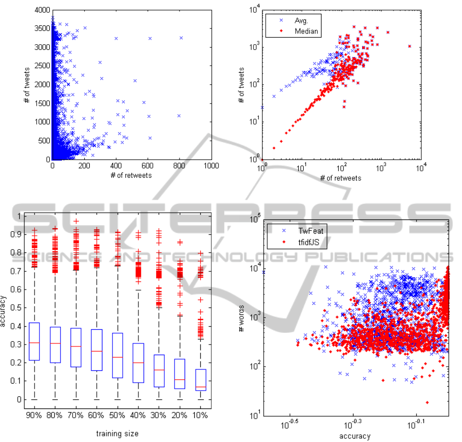
Figure 3: Number of tweets vs. number of retweets of each Twitter account.
Figure 4: Box plot showing the accuracy results for the dif-
ferent training set sizes tested.
standard BM25 and a version expanded with co-
occurrence of words by document using the for-
mula from Equation 10.
• Web-based Expansion. We implement the ap-
proach described in Section 2, where the terms are
expanded from search engine results. We query a
search engine for each short message of a Twitter
account and compute the tf-idf of the top-5 docu-
ments retrieved.
4.2 Results
Table 1 presents summary statistics for the accuracy
Figure 5: Accuracy results based on the number of unique
words of a Twitter account.
results of the tested models. Mean values are com-
puted across all Twitter accounts tested and all train-
ing sizes used. It shows slightly better performance
overall for the tf-idf model expanded with the Jensen-
Shannon method. All the methods to expand the tf-idf
model perfomed better than the traditional tf-idf and
BM25 models. After these two, the model with Twit-
ter features follows with the third worse accuracy. Fi-
nally, the Web-based expansion method has slightly
worse performance than the other methods of word
expansion tested.
Precision, on the other hand, as shown on Table 2
shows positive results for the tf-idf model expanded
with the Jensen-Shannon method. Precision, in this
WEBIST2013-9thInternationalConferenceonWebInformationSystemsandTechnologies
418

Table 1: Accuracy results for the different methods tested. tfidfJS is the tf-idf expanded with the Jensen-Shannon
method,tfidfCo is expanded with the word co-occurrence probabilities from Equation 9, tfidfDoc is expanded with the word
co-occurrence probabilities by message from Equation 10, TwFeat is the model with features from published messages and
WebExp is Web-based expansion approach described in Section 2.
tfidfJS tfidf tfidfCo tfidfDoc BM25 BM25Doc TwFeat WebExp
min 0.3339 0.1016 0.1016 0.1016 0.1016 0.1016 0.2607 0.2815
Q1 0.6078 0.3060 0.5150 0.6758 0.3060 0.6781 0.5886 0.5899
median 0.7898 0.5731 0.5731 0.7761 0.5731 0.7745 0.6704 0.7308
mean 0.7763 0.5310 0.5704 0.7557 0.5310 0.7560 0.6818 0.7422
Q3 0.9790 0.7158 0.6364 0.8787 0.7158 0.8786 0.7723 0.9222
max 0.9999 0.9509 0.9867 0.9989 0.9509 0.9989 0.9882 0.9997
std 0.1866 0.2438 0.1201 0.1661 0.2438 0.1657 0.1312 0.1811
Table 2: Precision results for the different methods tested.
tfidfJS tfidf tfidfCo tfidfDoc BM25 BM25Doc TwFeat WebExp
min 0.0079 0.0067 0.0256 0.0065 0.0205 0.0041 0.0159 0.0019
Q1 0.5542 0.1111 0.4308 0.1562 0.1112 0.1530 0.3920 0.2868
median 0.8889 0.2146 0.5342 0.2552 0.2222 0.2552 0.5593 0.6047
mean 0.7407 0.2189 0.5216 0.2839 0.2292 0.2829 0.5406 0.5875
Q3 1.0000 0.2222 0.6255 0.3843 0.2552 0.3825 0.7052 0.9017
max 1.0000 0.6667 1.0000 1.0000 0.6667 1.0000 1.0000 1.0000
std 0.3066 0.1564 0.1655 0.1691 0.1504 0.1695 0.2148 0.3241
case, measures how well the classifier identified the
“bad” tweets (i.e., the true positives), regardless of the
classification of normal tweets (i.e., the true and false
negatives). Classification using message features also
has a high precision compared with the poor accuracy
performance. We show later in Figure 7 that the clas-
sification using message features are further improved
with the addition of a time decay factor. Note also
the different standard deviation values of the models.
Although the tf-idf model expanded with the Jensen-
Shannon method has better accuracy and precision, its
standard deviation is significantly higher than in most
of the other models.
Differences in the results across the different mod-
els and even within the models could be explained by
different factors. First, a bigger training size yields
better classification. Figure 4 shows the overall av-
erage accuracy over all models grouped by training
size. The differences in the mean values, however,
is relatively small between training sizes of 50% and
90% of the messages, and specially between 70% and
90%. A more significant drop is seen for training sizes
of 40% or smaller. One reason for these differences
is the small number of retweets in many Twitter ac-
counts as shown in Figure 3. Hence, for training sets
very small, there is a high a chance that no “bad” mes-
sages are included in them. Similarly, for very large
training sets, chances are that all “bad” messages are
included in them, simplifying the classification of the
test set for those cases.
Another reason for the differences in the results
in the large variation in the number of unique words
present in a vector space model. Figure 5 plots the
number of unique words extracted from a Twitter ac-
count and the accuracy values for the model using
message features and expansions with the Jensen-
Shannon method. Note how accuracy increases with
the number of words for Jensen-Shannon method but
remains varied, regardless of the number of words for
the model of message features. The traditional tf-idf
model remains limited to the original set of words
while methods that expand it tend to improve over the
addition of new related or latent words. This could
explain the poor performance of certain types of ac-
counts. For example, inactive accounts with few but
similar messages and spam accounts that repeat the
publication of similar messages are more difficult to
model because the number of unique words tends to
be small.
A third reason that helps explain the variations in
the results is the total number of messages published
in a Twitter account as shown in Figure 6. The plots
are in log scale and represent respectively the average
accuracy and average precision per number of mes-
sages. In almost all cases, accuracy and precision are
higher in Twitter accounts with more messages pub-
lished. The notable exceptions are the accuracy and
precision of the tf-idf model and the precision of the
tf-idf model expanded with co-occurrency by docu-
ment. The poorer performance of the tf-idf could in-
ClassifyingShortMessagesonSocialNetworksusingVectorSpaceModels
419
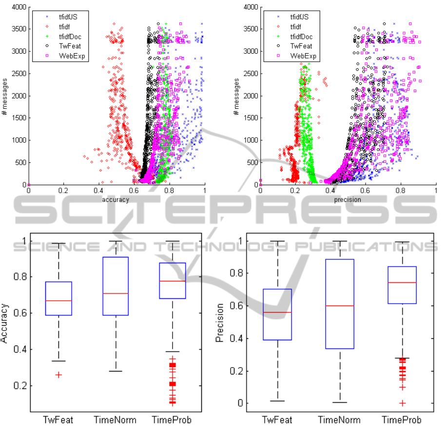
Figure 6: Accuracy and precision results of the tested models according to the number of messages of each account.
Figure 7: Box plots for accuracy and precision results of the following models: TwFeat (Twitter Features), TimeNorm (Twitter
Features plus normalized time difference) and TimeProb (Twitter Features plus each message’s p
m
(a|t) value).
dicate that the extra messages do not add relevant ex-
tra features for the classification. These new features
could be helpful to identify related or latent features
in other models but may not be useful by itself. In
the specific case of the BM25 approach, the similar
results to the tf-idf models could be explained by the
average document length of the tweets. Since most
tweets have similar lengths (and upper limit of 140
characters), the (N/avgdl) part of the S(Q = w) score
remains relatively unchanged. The score, then, boils
down to a tf-idf model with parameters that do not
seem to influence much the results.
Finally, the addition of a time decay feature helps
improve the classification. To test the addition of it,
we test two different time decay features on the orig-
inal model of Twitter Features. Figure 7 shows the
accuracy and precision results for the original model
of message features and two other with time decay
features. The first is a normalization of the time dif-
ference between a given message and the most re-
cent of that account and the second, our model, is a
probability measure of how likely a message is to be
retweeted. Results show that our model has on aver-
age better accuracy and precision that the other two
models tested.
WEBIST2013-9thInternationalConferenceonWebInformationSystemsandTechnologies
420

5 CONCLUSIONS AND FUTURE
WORK
In this paper we proposed a method based on vec-
tor space models to classify “bad” messages and pre-
vent their publication on a social network account.
We showed that the traditional tf-idf model performs
poorly due to the small amount of messages in each
account but it can improved with different expansion
techniques. We also tested different time decay pa-
rameters and showed that our model determined em-
pirically from a Twitter dataset performs best. Over-
all, it is feasible to train a classifier for this task and
reduce the amount of messages to evaluated for a rec-
ommendation process.
In future works, we plan to extend our method
testing it with different feature selection algorithms.
Furthemore, feature reduction could be performed
with co-occurence cluster analysis where attained
clusters would represent latent topics. These would
result into low-dimensional vector space with more
dense feature vectors that could help improve the clas-
sification further. We also plan to test how this classi-
fication could affect ranking algotihms aimed at rec-
ommending messages on a social network account.
REFERENCES
Chen, K., Chen, T., Zheng, G., Jin, O., Yao, E., and Yu, Y.
(2012). Collaborative personalized tweet recommen-
dation. In Proceedings of the 35th international ACM
SIGIR conference on Research and development in in-
formation retrieval, SIGIR ’12, page 661670, New
York, NY, USA. ACM.
Chen, M., Jin, X., and Shen, D. (2011). Short text classifica-
tion improved by learning multi-granularity topics. In
Proceedings of the Twenty-Second international joint
conference on Artificial Intelligence - Volume Volume
Three, IJCAI’11, page 17761781. AAAI Press.
Combarro, E., Montanes, E., Diaz, I., Ranilla, J., and
Mones, R. (2005). Introducing a family of linear
measures for feature selection in text categorization.
Knowledge and Data Engineering, IEEE Transactions
on, 17(9):1223–1232.
Dagan, I., Lee, L., and Pereira, F. C. N. (1999). Similarity-
based models of word cooccurrence probabilities.
Mach. Learn., 34(1-3):43–69.
D
´
ıaz, I., Ranilla, J., Monta
˜
nes, E., Fern
´
andez, J., and Com-
barro, E. (2004). Improving performance of text cat-
egorization by combining filtering and support vector
machines. Journal of the American society for infor-
mation science and technology, 55(7):579–592.
Halawi, G., Dror, G., Gabrilovich, E., and Koren, Y. (2012).
Large-scale learning of word relatedness with con-
straints. In Proceedings of the 18th ACM SIGKDD
international conference on Knowledge discovery and
data mining, KDD ’12, page 14061414, New York,
NY, USA. ACM.
Kwak, H., Lee, C., Park, H., and Moon, S. (2010). What
is twitter, a social network or a news media? In
Proceedings of the 19th international conference on
World wide web, pages 591–600, Raleigh, North Car-
olina, USA. ACM.
Lage, R., Durao, F., and Dolog, P. (2012). Towards effective
group recommendations for microblogging users. In
Proceedings of the 27th Annual ACM Symposium on
Applied Computing, SAC ’12, pages 923–928, New
York, NY, USA. ACM.
Lan, M., Tan, C.-L., Low, H.-B., and Sung, S.-Y. (2005).
A comprehensive comparative study on term weight-
ing schemes for text categorization with support vec-
tor machines. In Special interest tracks and posters of
the 14th international conference on World Wide Web,
WWW ’05, page 10321033, New York, NY, USA.
ACM.
Lewis, D. D. (1998). Naive (Bayes) at forty: The indepen-
dence assumption in information retrieval. In Ndel-
lec, C. and Rouveirol, C., editors, Machine Learning:
ECML-98, number 1398 in Lecture Notes in Com-
puter Science, pages 4–15. Springer Berlin Heidel-
berg.
Lin, J. and Mishne, G. (2012). A study of ”Churn” in tweets
and real-time search queries. In Sixth International
AAAI Conference on Weblogs and Social Media.
Mladenic, D. and Grobelnik, M. (1999). Feature selec-
tion for unbalanced class distribution and naive bayes.
In Machine Learning-International Workshop Then
Conference-, pages 258–267. Morgan Kaufmann Pub-
lishers, Inc.
Petrovic, S., Osborne, M., and Lavrenko, V. (2011). RT
to win! predicting message propagation in twitter. In
Fifth International AAAI Conference on Weblogs and
Social Media.
Robertson, S. E., Walker, S., Beaulieu, M., and Willett, P.
(1998). Okapi at TREC-7: automatic ad hoc, filtering,
VLC and interactive track. In TREC, pages 199–210.
Sahami, M. and Heilman, T. D. (2006). A web-based ker-
nel function for measuring the similarity of short text
snippets. In Proceedings of the 15th international con-
ference on World Wide Web, WWW ’06, page 377386,
New York, NY, USA. ACM.
Sun, A. (2012). Short text classification using very few
words. In Proceedings of the 35th international ACM
SIGIR conference on Research and development in in-
formation retrieval, SIGIR ’12, page 11451146, New
York, NY, USA. ACM.
Turney, P. D. and Pantel, P. (2010). From frequency
to meaning: Vector space models of semantics.
arXiv:1003.1141. Journal of Artificial Intelligence
Research, (2010), 37, 141-188.
Yang, Y. and Pedersen, J. (1997). A comparative study on
feature selection in text categorization. In Machine
Learning-International Workshop Then Conference-,
pages 412–420. Morgan Kaufmann Publishers, Inc.
Yih, W.-t., Goodman, J., and Carvalho, V. R. (2006). Find-
ing advertising keywords on web pages. In Proceed-
ings of the 15th international conference on World
ClassifyingShortMessagesonSocialNetworksusingVectorSpaceModels
421

Wide Web, WWW ’06, page 213222, New York, NY,
USA. ACM.
Yih, W.-T. and Meek, C. (2007). Improving similarity mea-
sures for short segments of text. In Proceedings of the
22nd national conference on Artificial intelligence -
Volume 2, AAAI’07, page 14891494. AAAI Press.
WEBIST2013-9thInternationalConferenceonWebInformationSystemsandTechnologies
422
