Optimized Cascade of Classifiers for People Detection using Covariance
Features
Malik Souded
1,2
and Francois Bremond
1
1
STARS Team, INRIA Sophia Antipolis - M´editerran´ee, Sophia Antipolis, France
2
Digital Barriers France, Sophia Antipolis, France
Keywords:
People Detection, Covariance Descriptor, LogitBoost.
Abstract:
People detection on static images and video sequences is a critical task in many computer vision applications,
like image retrieval and video surveillance. It is also one of most challenging task due to the large number of
possible situations, including variations in people appearance and poses. The proposed approach optimizes an
existing approach based on classification on Riemannian manifolds using covariance matrices in a boosting
scheme, making training and detection faster while maintaining equivalent performances. This optimisation
is achieved by clustering negative samples before training, providing a smaller number of cascade levels and
less weak classifiers in most levels in comparison with the original approach. Our work was evaluated and
validated on INRIA Person dataset.
1 INTRODUCTION
Person detection is one of the most challenging task
in computer vision. The large variety of people poses
and appearences, added to all external factors like dif-
ferent points of view, scenes content and partial occlu-
sions make this issue complicated. The importance
of this task for many applications like people track-
ing especially in crowded scenes has motivated many
researches. A lot of approaches were proposed as re-
sults of these research.
The most frequent scheme consists in using de-
scriptors to modelize a person. To perform this mod-
elization, an offline learning step is carried using these
descriptors. Once the learning achieved and the clas-
sifier obtained, the detection is performed by testing
all possible image subwindows.
In (Papageorgiou and Poggio, 2000), Papageor-
giou and Poggio used Haar-like features to train a
SVM classifier. Viola et al. (Viola et al., 2006) trained
a cascade of Adaboost classifiers using Haar-like fea-
tures too. In (Dalal and Triggs, 2005), a new descrip-
tor called Histogram of Oriented Gradients (HOG)
was introduced by Dalal and Triggs and was used to
train a linear SVM, providing very good people detec-
tor. Dala et al. associate this descriptor later in (Dalal
et al., 2006) with histograms of differential optical
flow features outperforming the previous approach.
Mu et al. have proposed new variants of
well known standard LBP descriptor in (Mu et al.,
2008). They demonstrated the effectiveness of their
Semantic-LBP and Fourier-LBP features in com-
parison to standard LBP for people detection. In
(Schwartz et al., 2009), Schwartz et al. concatained
HOG, color frequency and co-occurence matrices as
one descriptor and employed Partial Least Square
analysis for dimensionality reduction.
All the previous mentioned approaches can be
classified as dense representation methods due to the
detection method (dense search on images). Some
other approaches use different detection method
and can be categorized as sparse representation ap-
proaches. They consists of modeling the human body
parts, detect them and achieve people detection using
geometric constrains. In (Mikolajczyk et al., 2004),
dedicated Adaboost detectors were trained for several
body parts. The final detection is obtained by opti-
mizing the likelihood of part occurence along with the
geometric relation.
Recently, Tuzel et al. (Tuzel et al., 2007) propose
a performant approach for people detection. Their
approach uses covariance descriptors to characterise
people. This characterisation is achieved by training
a cascade of classifiers on a dataset containing human
and non-human images. The training is done using
a modified version of LogitBoost algorithm to deal
with some specificities and constraints of covariance
descriptors. One of the main covariance descriptor
820
Souded M. and Bremond F..
Optimized Cascade of Classifiers for People Detection using Covariance Features.
DOI: 10.5220/0004304208200826
In Proceedings of the International Conference on Computer Vision Theory and Applications (VISAPP-2013), pages 820-826
ISBN: 978-989-8565-47-1
Copyright
c
 2013 SCITEPRESS (Science and Technology Publications, Lda.)

issues is the computing time of all related operators
and metrics. It makes covariance descriptors difficult
to use for real-time processing.
Yao and Odobez (Yao and Odobez, 2008) have
proposed three main contributions to this approach
improving the efficiency of the training and detection
stage, and providing better performances.
Because our approach is mainly based on these
two last approaches, a brief recall about covariance
descriptor computation, and a summary of the two
cited approaches are described below.
The two approaches present some issues. In the
next section, the main contribution of this paper,
addressing these issues, is presented. Finally, the
experimental results demonstrate that the proposed
approach provides equivalent performances that the
original ones while improving the processing time of
the training and detection stage.
2 PEOPLE DETECTION USING
COVARIANCE FEATURES
2.1 Region Covariance Descriptor
Region covariance descriptor is a powerful way to en-
code a large amount of information inside in a given
image region. Il allows the encapsulation of a large
range of different features in a single structure, repre-
senting the variances of each feature and the correla-
tion between features.
Let I be an image of dimension W ×H. We can
extract at each pixel location x = (x, y)
T
a set of d
features such as intensity, color, gradients, filter re-
sponses, etc.
For a given rectangular region R of I, let {z
i
}
i..S
be
the d-dimensional feature points inside R. The region
R is represented with the d ×d covariance matrix of
the feature points
C
R
=
1
S−1
S
∑
i=1
(z
i
−µ)(z
i
−µ)
T
(1)
where µ is the mean of the points z
i
and S the number
of pixels within R
2.1.1 Used Features
In (Tuzel et al., 2007), Tuzel et al. use a 8-
dimensional set of features

x y |I
x
| | I
y
|
q
I
2
x
+ I
2
y
|I
xx
| |I
yy
| arctan
|I
x
|
|I
y
|

T
(2)
where x and y are the pixel location, I
x
;I
xx
;... are in-
tensity derivatives, and the last term is the gradient
orientation.
Yao and Odobez (Yao and Odobez, 2008) replace
the two second derivatives features |I
xx
| and |I
yy
| by
two foreground measures G and
q
G
2
x
+ G
2
y
. G
denotes the foreground probability value (a real num-
ber between 0 and 1 indicating the probability that the
pixel x belongs to the foreground), and G
x
and G
y
are the corresponding first order derivatives. These
foreground features are obtained using a background
subtraction technique which is restricted to moving
people. These two features improve people detec-
tion performances and processing time in video se-
quences.
2.1.2 Fast Covariance Descriptor Computation
A large number of covariance descriptors are required
to achieve the training of classifier cascade and for an
effective process. The computation of all the feature
sums, means and variances for each region has a high
cost in term of processing time. To deal with this, In-
tegral images are ideally suited to minimize the num-
ber of numerical operations.
Integral images are intermediate image represen-
tations used for the fast calculation of region sums
(Simard et al., 1998), (Viola and Jones, 2001). Each
pixel of the integral image is the sum of all the pixels
inside the rectangle bounded by the upper left corner
of the image and the pixel of interest.
Due to the symmetic nature of covariance matri-
ces, only upper (or lower) triangle values are needed.
In the case of 8-feature set, the covariance matrix will
contain 36 different values, and 44 Integral Images
are computed to speed up the computing process (8
integral images for the representation of each feature
independently and 36 for the representation of prod-
uct for each pair of features).
2.1.3 Covariance Normalisation
In order to enhance covariance descriptors robustness
toward local illumination changes, a normalization
step is performed on the covariance matrix. Let r be a
subregion contained in a larger region of interest R.
First, both covariance matrices C
r
and C
R
are
computed using integral representation. After that,
the values of covariance matrix C
r
are normalized
with respect to the standard deviations of their cor-
responding. features inside the detection window R
as in (Tuzel et al., 2007) The normalized covariance
descriptor is denoted
ˆ
C
r
.
OptimizedCascadeofClassifiersforPeopleDetectionusingCovarianceFeatures
821

2.1.4 LogitBoost Algorithmon Riemannian
Manifolds
The classification process is performed using a
cascade of classifiers which is trained using a
LogitBoost algorithm on Riemannian Manifolds.
Standard LogitBoost Algorithm on Vector Spaces.
As seen in (Friedman et al., 2000), let {(x
i
, y
i
)}
i=1...N
be the set of training samples, with y
i
∈ {0, 1} and
x
i
∈ R
n
. The goal is to find a decision function F
which divides the input space into the 2 classes. In
LogitBoost, this function is defined as a sum of weak
classifiers, and the probability of a sample x being in
class 1 (positive) is represented by
p(x) =
e
F(x)
e
F(x)
+ e
−F(x)
, F(x) =
1
2
N
L
∑
l=1
f
l
(x). (3)
The LogitBoostalgorithmiteratively learns the set
of weak classifiers {f
l
}
l=1...N
L
by minimizing the neg-
ative binomial log-likelihood of the training data:
−
N
∑
i
[y
i
log(p(x
i
)) + (1−y
i
)log(1− p(x
i
))], (4)
through Newton iterations. At each iteration
l, this is achieved by solving a weighted least-
square regression problem:
∑
N
i=1
w
i
kf
l
(x
i
) −z
i
k
2
,
where z
i
=
y
i
−p(x
i
)
p(x
i
)(1−p(x
i
))
denotes the re-
sponse values, and the sample weights
are given by w
i
= p(x
i
)(1 − p(x
i
)).
LogitBoost Algorithm on Riemannian Manifolds.
To train classifiers using covariance descriptors, this
algorithm is not usable as it is. In fact, covariance
descriptors do not belong to vector spaces but to the
Riemannian manifold M of d ×d symmetric positive
definite matrices Sym
+
d
.
Based on an invariant Riemannian metric on the
tangent space defined in (Pennec et al., 2006), let X
and Y be two matrices from Sym
+
d
, the following op-
erators are defined and used to achieve training using
LogitBoost on Riemannian manifold:
exp
X
(y) = X
1
2
exp(X
−
1
2
yX
−
1
2
)X
1
2
(5)
log
X
(y) = X
1
2
log(X
−
1
2
yX
−
1
2
)X
1
2
(6)
d
2
(X, Y) = trace

log
2
(X
−
1
2
YX
−
1
2
)

(7)
which are respectively the exponential, the loga-
rithm and the squared distance on Sym
+
d
matrices.
exp(y) = U exp(D)U
T
and log(y) = U log(D)U
T
.
y = UDU
T
is the eigenvalue decomposition of the
symmetric matrix y and exp(D) and log(D) are ob-
tained by applying exponential and logarithm func-
tions respectively on the diagonal entries of the diag-
onal matrix D.
Tuzel et al. have introduced a modifications to the
original LogitBoost algorithm to specifically account
for the Riemannian geometry. This was done byintro-
ducing a mapping function h projecting the input co-
variance descriptors into the Euclidian tangent space
at a point µ
l
of the manifold M :
h(X) = vec
µ
l
(log
µ
l
(X)) (8)
where: vec
X
(y) = vec
I
(X
−
1
2
yX
−
1
2
), and vec
I
(y) =
[y
1,1
√
2y
1,2
√
2y
1,3
... y
1,2
√
2y
2,3
... y
d,d
]
T
.
The trained cascade consists of a list of ordered
strong classifiers. Each strong classifier contains a set
of weak classifiers. A weak classifier is defined by a
sub-region of interest, the corresponding mean value
of covariance descriptors of all positive samples and
a regression function.
To train a level k of the cascade, a given number
of weak classifiers are successively added. To add a
weak classifier l to the current training classifier, 200
candidate weak classifiers are evaluated: 200 subwin-
dows are randomly selected. Let r
i
be one of these
subwindows and
ˆ
C
j
r
i
the corresponding normalized
covariance descriptor on the sample j. For each sub-
region r
i
, the mean µ
i
of all the normalized covariance
descriptors
ˆ
C
j
r
i
of the positive samples is computed
using a gradient descent procedure described in (Pen-
nec et al., 2006). Using this mean µ
i
, all
ˆ
C
j
r
i
of all
the samples are projected onto the tangent space using
(8) obtaining vectors in Euclidean space. Using these
vectors and the corresponding weights of all samples,
a regression fucntion g
i
is computed.
The best weak classifier, which minimizes nega-
tive binomial log-likelihood (4), is added to the cur-
rent training classifier. The weights and the proba-
bilities of all the samples are updated according to
the new added weak classifier. The positive and the
negative samples are sorted in a decreasing order us-
ing their probabilities. The current strong classifier is
concidered as fully trained if the difference between
the probability of the (99.8%)
th
positive sample and
the (35%)
th
negative sample is greater than 0.2.
In this case, the training of the current cascade
level is achieved. The negative samples are tested
with the new cascade and all correctly classified sam-
ples are removed from the training dataset. The next
cascade level is trained using remaining negatives.
VISAPP2013-InternationalConferenceonComputerVisionTheoryandApplications
822

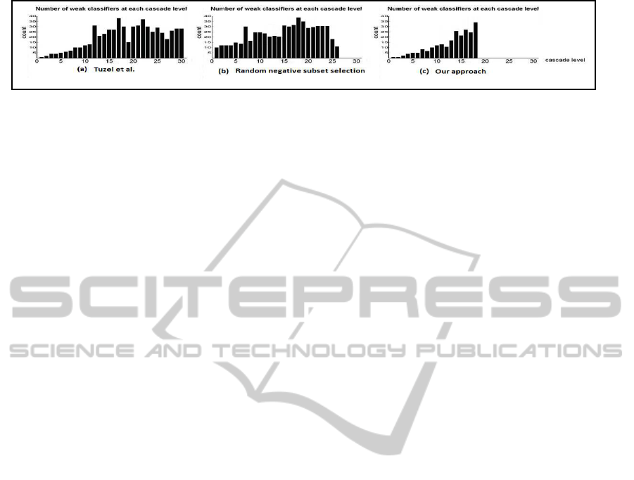
Figure 1: Comparison between structures of the cascade of classifiers: (a) Tuzel et al.(Tuzel et al., 2007); (b) trained with a
random selection of negative subset; (c) our proposed approach: less cascade levels with less weak classifiers per level.
Note that Yao et. al have introduced two impor-
tant improvements. First, classifiers are trained on a
lower dimension. They proposed an approach to se-
lect the best subset of d
′
features from the d origi-
nal ones for each sub-region. They train classifiers on
4-feature covariance descriptors. Second, they have
concatained the mean feature vector of each random
sub-region to the mapped vector of each sample be-
fore regression computing, improving performances.
2.2 Main Issues
The initial approach proposed by Tuzel et al. (Tuzel
et al., 2007) outperforme existing approaches of the
state of the art by providing a lower rate of miss-
detections and false positives, but it has the disadvan-
tage of being highly time consuming for the detection
process and not applicable for real-time processing.
In (Tuzel et al., 2007), Tuzel et al. indicate that detec-
tion time on a 320 x 240 image is approximatively 3
seconds for a dense scan, with 3 pixel jumpsvertically
and horizontally. Note that training time is relatively
long also (2 days in (Tuzel et al., 2007)).
The most computationnally expensive operation
during the training and the classification is eigenvalue
decomposition. This decomposition is the basis of all
operators in Sym
+
d
. Eigenvalue decomposition of a
symmetric d ×d matrix requires O(d
3
) arithmetic op-
erations, so computing time increases quickly by us-
ing more features.
The feature subset selection approach, proposed
by Yao and Odobez in (Yao and Odobez, 2008) al-
lows to work in a lower dimensional symmetric posi-
tive definite matrices, making eigenvalue decomposi-
tion faster and thereby improving all the training and
classification processes.
We focus in our work on another way to make the
classification faster while maintaining high classifica-
tion performances. At the end, the obtained approach
improve also the training stage.
3 PROPOSED ALGORITHM
3.1 Ordering Negative Training Sample
Using large number of samples for the training pro-
cess makes it very slow. Of course, the larger the
training dataset is, the more performant the classifier
cascade is. But most of the time, large number of neg-
ative samples contain very similar information. This
problem is more frequent for the first cascade levels,
where a new level is trained using false positives of
previous levels. These false positives are generally
resulting from successive small shifts of testing win-
dow on the image, providing very similar content.
One can suppose that using a smaller subset of
randomly selected negative samples to train a given
cascade level can be a good solution to speed up train-
ing. We can suppose that a randomly selected sub-
set can be statistically representative of all remaining
negatives.
We have tested this approach and we have ob-
served that it effectively speeds up training and pro-
vides a lower number of cascade levels than (Tuzel
et al., 2007) but with longer classifiers (See Figure. 1,
b), slowing down in comparison to the previous men-
tioned approaches. In fact, one cascade level consists
of a set of weak classifiers. The response of one clas-
sifier is obtained after computing the output values of
all its weak classifiers. It means than a long classifier
containing a large number of weak classifiers takes
more time to return a decision, so a cascade of long
classifiers is very slow for detection.
The number of weak classifiers per cascade level
depends mainly on the diversity of negative samples
used for the training. The characterisation of positives
and their separation from negativesl requires as many
subregions of interest as the samples are diverse.
To illustrate the relationship between negative
samples diversity and classifiers cascade structure, let
us use a simple example which can be generalized to
understand the concept. Suppose that we have to sep-
arate a person image from three non-person images:
a sky image, a vertical barrier image and a lamppost
OptimizedCascadeofClassifiersforPeopleDetectionusingCovarianceFeatures
823

93.53 50.04 52.84 66.46
49.36 15.91 13.84 38.50
8.97 8.62 7.42 11.50
4.86 5.45 8.31 19.26
Negative
Sample 1
Negative
Sample 2
Negative
Sample 1
Negative
Sample 3
d²(X, Y) per
sub-region
191.68 23.04 92.84 30.31
49.50 14.80 9.71 53.18
17.71 34.37 94.11 39.31
31.78 26.85 105.85 76.81
d²(X, Y) per
sub-region
d² = 454.87
d² = 891.87
the squared
distance between
the two samples
the squared
distance between
the two samples
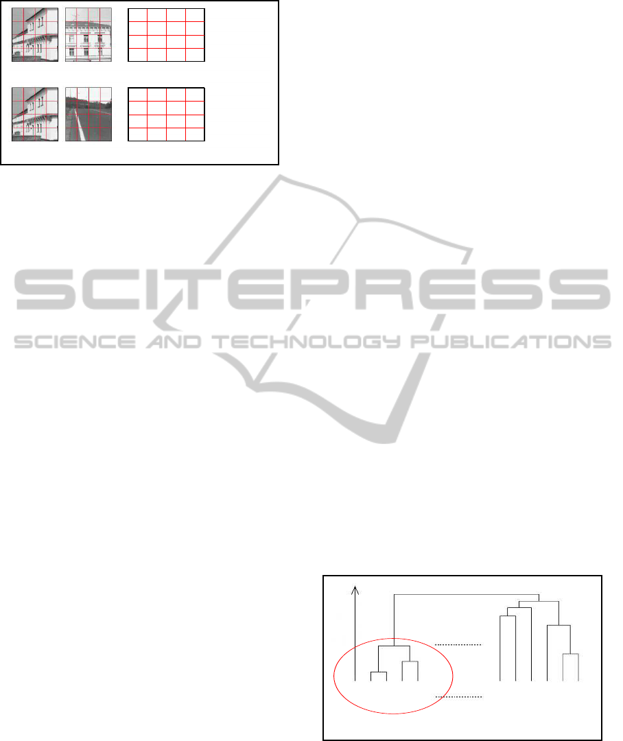
Figure 2: Used Squared distance computation between two
negative samples for hierarchical clustering.
image. Due to the poverty of texteures and gradiends
on the sky image, a unique large covariance region
is sufficient to separate the sky image from the per-
son image, which has many gradients and a vertical
shape. For vertical barriers, the previous region is not
appropriate due to the vertical shape of the person. A
smaller region around the person’s head is more ap-
propriate. The circular shape of the head provides a
good separation. Now, for the lamppost, the two pre-
vious regions are not suitable. It is necessary to take
a region on legs or around shoulders to encode cur-
vatures. For this example, there are two methods to
train the classifier. The first cascade is trained with
one negative image at a time in the mentionned order.
The second cascade is trained with the three negative
images at the same time, using approriate parameters.
The first method provides a cascade with three levels,
each level containing one weak classifier corresopnd-
ing to onecase (low texture level, vertical shapes only,
circular shape at the top of vertical shape). The sec-
ond method provides a cascade of a unique classifier
containing three weak classifiers at least (the number
can be larger du to the possible combinations).
Suppose now that we have to perform a people
detection on a large image which contains only sky,
a low textured road, some vertical barriers and some
lampposts. Both cascades will provide equivalent de-
tection performances, but the first one will be faster.
This is becausemost of tested windows (sky and road)
are rejected after evaluating only one covariance de-
scriptor (the one of the first cascade level), while the
second classifier cascade needs to evaluate three (or
more) covariance descriptors for each tested window.
The average number of evaluated covariance de-
scriptors using Tuzel et al. cascade (a) is 8.45 while
the cascade in (b) needs more than 21 covariance de-
scriptor evaluation.
We propose an approach using a shorter subset
of negatives at each cascade level training to make
it faster. Our approach provides shorter cascade with
smaller classifiers on average (Figure. 1, c ) in com-
parison with the Tuzel et al. one (Figure. 1, a) mak-
ing detection process faster. At the same time, the
experimental results show that our approach provides
similar detection performances than the original one.
3.2 Clustering on Negative Data
The idea consists in regrouping negative samples per
groups containing similar contents in terms of co-
variance information, and train each cascade level by
one group of similar samples. The previously de-
scribed Logitboost algorithm achieves characteriza-
tion of people against a group of negative samples
faster when these negative samples are more similar.
It also specialize each cascade level. This negative
samples regrouping is achievd using clustering meth-
ods. We tried two methods to perform this clustering,
the first one is applyed directely in Riemannian man-
ifold while the second one is performed in the Eu-
clidean space.
3.2.1 Hierarchical Clustering on Covariance
Descriptors using Covariance Matrices
Distance
A matrix containing the distances between all pairs of
negative samples is computed. To compute the dis-
tance between two negative samples using covariance
descriptors, each sample image is divided into a grid
of 16 equal sub-regions. The final distance between
the two samples is the sum of the 16 distances be-
tween each covariance descriptors pair using (7) (See
Figure. 2). Once the distance matrix computed, a hi-
erarchcal clustering is performed, providing a tree of
negative samples (See Figure. 3)
Distance
Sample 1 Sample 2 Sample 3 Sample 4
Sample N-5 Sample N-4 Sample N-3 Sample N-2 Sample N-1 Sample N
Negative samples
Cluster of 35% of
Negative samples
Figure 3: Hierarchical tree of clustered negative samples.
3.2.2 Clustering in Projection Space
The second clustering approach consists in project-
ing all negative samples to a tangent space. In this
method, we use covariance descriptor of the whole
VISAPP2013-InternationalConferenceonComputerVisionTheoryandApplications
824

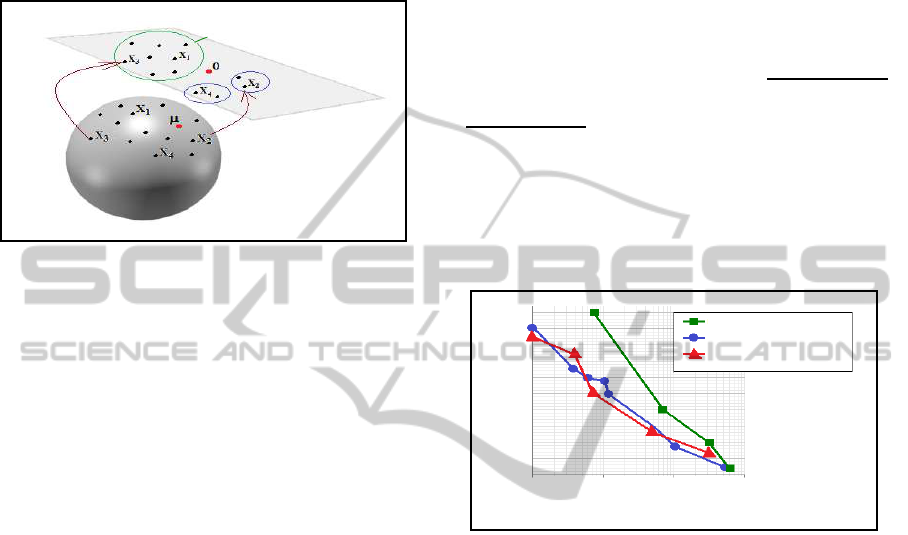
image of each sample. The mean of all negative
samples is computed and used to project all covari-
ance descriptors to the Euclidean space. Finally Eu-
clidean space, the clustering is performed using adap-
tive bandwidth mean shift filtering (Comaniciu and
Meer, 2002). (See Figure. 4)
Largest cluster
log
µ
log
µ
M
Figure 4: Clustering on tangent space.
3.3 Train Iteratively by each Subset
After clustering, it is now possible to select the n most
similar negatives samples. In the case of hierarchical
clustering, we select first the cluster which contain n
= 35 % of remaining negatives. we took this value ac-
cording to Tuzel et al. parameters (Tuzel et al., 2007),
to have similar conditions and to be able to compare
results. In the mean shift clustering on tangent space,
we select the cluster containing the largest number of
samples. This is motivated by the desire to eliminate
the largest percentage of negative samples as soon as
possible.
The training is now done by applying a cluster-
ing step on the negative samples, selecting the most
similar negatives subset and use it for training. After
achieving current level training, the new cascade is
applyed to all the remaining negative samples, those
used for training and the others. We observed that
80% to 95% of the negatives from the used subset are
correctly classified and removed and a small part of
unused negatives too.
The clustering is repeated on remaining negatives
to train next levels.
4 EXPERIMENTAL RESULTS
We conduct experiments on INRIA dataset to be able
to compare our results with those of Tuzel et al.
(Tuzel et al., 2007).
The INRIA person dataset (Dalal and Triggs,
2005) is devided to two subsets: a training set con-
taining 2416 person annotationsand 1218 person-free
images and a test dataset with 1132 persons ans 453
person-free images. This dataset is quite challenging
due to the various scenes, content, and persons ap-
pearence and poses.
4.1 Detection Performances
Comparison
The detection performances were evaluated on two
criteria: miss detection rate, given by
FalseNeg
FalseNeg+TruePos
and false positive per window, which is given by
FalsePos
TrueNeg+FalsePos
. The rightmost curve points of our
method corresponds to the results of the 8 first levels
of the cascade. The other points are added every 4
cascade levels. The curve in Figure 5 show that our
approach provides very close performances to Tuzel
et al. ones, which outperform Dalal et al. results
(Dalal et al., 2006)
0.01
0.02
0.04
0.06
0.08
0.1
10
-5
10
-4
10
-3
10
-2
Dalal et al. : Ker SVM
Tuzel et al. : LogitBoost on Sym
8
+
Our approach : Clustering+
LogitBoost on Sym
+
8
miss rate
false positives per window (FPPW)
Figure 5: Comparison with the methods of Dalal et al.
(Dalal et al., 2006) and Tuzel et al. (Tuzel et al., 2007)
on the INRIA data set.
4.2 Classifier Cascade Structure,
Training Time and Detection Time
Comparison
Our cascade of classifier (See Figure. 1 (c)) is shorter
than the Tuzel et al. one. It contains 18 levels achiev-
ing rejection of more than 99% of negatives during
training. Most levels contain less weak classifiers
also. The average number of evaluated covariance de-
scriptors using our cascade is 6.85 while it is 8.45 for
Tuzel et al. cascade
The main consequence of this difference of struc-
tures is the detection time. Our cascade perform de-
tection faster than the Tuzel el al. one. We have im-
plemented both approaches with C++ and performed
training and detection on an Intel(R) Core(TM) i7-
920 Processor at 2.66-Ghz with 4Gbytes or RAM.
The average time of detection on images of 320x240
is approximatively 2.3 seconds for Tuzel et al. while
it is approximatively 0.5 seconds for our method.
OptimizedCascadeofClassifiersforPeopleDetectionusingCovarianceFeatures
825

In the same conditions, training time is also de-
creased by our approach. The training takes 22 hours
for Tuzel et al. approach while it takes 9 hours for our
approach.
Note finally that the clustering in tangent space
provide better results for first cascade levels training,
but after few levels, it becomes less precise. This can
be explained by the fact that at the first level,negative
samples are densly regrouped. The computed mean
for tangent space projection is significant. After few
level training, and removing correct classified neg-
atives, the remaining negatives became sparse and
computing a mean on sparse samples make it less sig-
nicative, the projection to tangent space is not suit-
able.
5 CONCLUSIONS
We have proposed an approach to optimize people de-
tection using covariance descriptors. This approach
consists in clustering negative data before training to
obtain better classifier structure. The resulting de-
tector is faster that original one and was trained in
shorter time. The experimental results on a challeng-
ing dataset validate our approach.
REFERENCES
Comaniciu, D. and Meer, P. (2002). Mean shift: A robust
approach toward feature space analysis. IEEE Trans.
Pattern Anal. Machine Intell., 24:603619.
Dalal, N. and Triggs, B. (2005). Histograms of oriented
gradients for human detection. In IEEE Conf. Comp.
Vision and Pattern Recognition (CVPR).
Dalal, N., Triggs, B., and Schmid, C. (2006). Human de-
tection using oriented histograms of flow and appear-
ance. In Europe Conf. Comp. Vision (ECCV), volume
II, pages 428441.
Friedman, J., Hastie, T., and Tibshira, R. (2000). Additive
logistic regression: a statisticalview of boosting. Ann.
Statist., 23(2):337C407.
Mikolajczyk, K., Schmid, C., and Zisserman, A. (2004).
Human detection based on a probabilistic assembly of
robust part detectors. In Europe Conf. Comp. Vision
(ECCV), volume I, pages 6981.
Mu, Y., Yan, Y., Liu, Y., Huang, T., and Zhou, B. (2008).
Discriminative local binary patterns for human detec-
tion in personal album. In CVPR 2008, pages 18.
Papageorgiou, P. and Poggio, T. (2000). A trainable sys-
tem for object detection. Int. J. of Computer Vision,
38(1):1533.
Pennec, X., Fillard, P., and Ayache, N. (2006). A rieman-
nian framework for tensor computing. Int. Journal of
Comp. Vision, 66(1):4166.
Schwartz, W., Kembhavi, A., Harwood, D., and Davis, L.
(2009). Human detection using partial least squares
analysis. In ICCV.
Simard, P., Bottou, L., Haffner, P., and LeCun, Y. (1998).
Boxlets: A fast convolution algorithm for signal pro-
cessing and neural networks. Proc. Conf. Advances
in Neural Information Processing Systems II, pp. 571-
577.
Tuzel, O., Porikli, F., and Meer, P. (2007). Human detection
via classification on riemannian manifolds. In IEEE
Conf. Comp. Vision and Pattern Recognition (CVPR).
Viola, P. and Jones, M. (2001). Rapid object detection
using a boosted cascade of simple features. Proc.
IEEE Conf. Computer Vision and Pattern Recognition
(CVPR 01), vol. 1, pp. 511-518.
Viola, P., Jones, M., and Snow, D. (2006). Detecting pedes-
trians using patterns of motion and appearance. In Eu-
rope Conf. Comp. Vision (ECCV), volume II, pages
589600.
Yao, J. and Odobez, J. (2008). Fast human detection from
videos using covariance feature. In: ECCV 2008 Vi-
sual Surveillance Workshop.
VISAPP2013-InternationalConferenceonComputerVisionTheoryandApplications
826