Unsupervised Feature Learning using Self-organizing Maps

Marco Vanetti, Ignazio Gallo and Angelo Nodari

Dipartimento di Scienze Teoriche e Applicate, Universit

a degli Studi dell’Insubria, Varese, Italy

Keywords:

Unsupervised Feature Learning, Self-organizing Map, Natural Images Classiﬁcation.

Abstract:

In recent years a great amount of research has focused on algorithms that learn features from unlabeled data.

In this work we propose a model based on the Self-Organizing Map (SOM) neural network to learn features

useful for the problem of automatic natural images classiﬁcation. In particular we use the SOM model to

learn single-layer features from the extremely challenging CIFAR-10 dataset, containing 60.000 tiny labeled

natural images, and subsequently use these features with a pyramidal histogram encoding to train a linear SVM

classiﬁer. Despite the large number of images, the proposed feature learning method requires only few minutes

on an entry-level system, however we show that a supervised classiﬁer trained with learned features provides

signiﬁcantly better results than using raw pixels values or other handcrafted features designed speciﬁcally for

image classiﬁcation. Moreover, exploiting the topological property of the SOM neural network, it is possible

to reduce the number of features and speed up the supervised training process combining topologically close

neurons, without repeating the feature learning process.

1 INTRODUCTION

For some very complex problems, such as the au-

tomatic categorization of natural images, a common

trend in recent years consists in the use of unsuper-

vised feature learning and deep learning algorithms

to learn a set of features from unlabeled data in an un-

supervised approach. Features learned are typically

used to train a supervised discriminative model, e.g.

a SVM classiﬁer. Feature learning algorithms are op-

posed to methods that use speciﬁc handcrafted fea-

tures, chosen by a domain expert. In deep learning lit-

erature many methods such as K-means and Gaussian

Mixtures (Coates et al., 2011), Autoencoder (Hin-

ton and Salakhutdinov, 2006; Bengio et al., 2007),

Restricted Boltzmann Machine (Hinton et al., 2006;

Krizhevsky, 2009) and Sparse Coding (Lee et al.,

2006) have been successfully applied to the problem

of single-layer feature learning and multi-layers deep

learning. Even in the computer vision literature have

been proposed methods that exploit the K-means al-

gorithm to create a dictionary of visual words used

as a feature in many visual class recognition prob-

lems (Lazebnik et al., 2006; Csurka et al., 2004).

In this work we train a Self-Organizing Map

(SOM) neural network to learn single-layer features

from the extremely challenging CIFAR-10 dataset,

containing 60.000 tiny natural images belonging to

10 classes, with 6.000 images per class (Krizhevsky,

2009). In the experimental section we show that a

supervised linear SVM classiﬁer trained with oppor-

tunely encoded learned features provides signiﬁcantly

better results than using raw pixels values or the Pyra-

mid Histogram of Oriented Gradients (PHOG), a pop-

ular handcrafted feature used in computer vision to

represent the shape of objects and to perform vi-

sual class recognition in natural images (Bosch et al.,

2007b; Bosch et al., 2007a). Contrary to most feature

learning algorithms, the proposed method is fast and

requires just few minutes to train the SOM, despite

the large number of images involved in the process.

The major contribution of this work is the empir-

ical study of the SOM neural network used to learn

features from a very big and challenging datasets,

the CIFAR-10. The unsupervised learning process

is fast and can be controlled by adjusting the size

of the SOM. Moreover our results show that using

the proposed method it is possible to arbitrarily re-

duce the number of features without repeating the

feature learning process by combining topologically

close neurons. This interesting property follows di-

rectly from the topological ordering property of the

SOM neural network.

This work is organized as follow. In Section 2.1

we describe the unsupervised feature learning model,

based on the SOM neural network, while Section 2.2

deals with the encoding of learned features. In Sec-

tion 3 are shown and discussed experimental results

596

Vanetti M., Gallo I. and Nodari A..

Unsupervised Feature Learning using Self-organizing Maps.

DOI: 10.5220/0004210305960601

In Proceedings of the International Conference on Computer Vision Theory and Applications (VISAPP-2013), pages 596-601

ISBN: 978-989-8565-47-1

 2013 SCITEPRESS (Science and Technology Publications, Lda.)

...

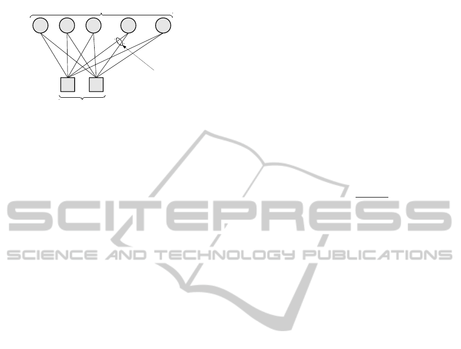
Input layer

Neurons

Weighted link

=[w

, … ,

]

1 2 3 i m

... ...

Figure 1: One-dimensional SOM.

obtained on the CIFAR-10 dataset. Finally, Section 4

gives the conclusions.

2 THE PROPOSED METHOD

This section describes the feature learning phase, per-

formed by the SOM on a large set of images, and the

encoding that exploits these learned features to de-

scribe a new image.

2.1 Unsupervised Feature Learning

As discussed in Section 1, the proposed method is

based on the SOM, an artiﬁcial neural network ﬁrst

proposed by Teuvo Kohonen in early 1981. This neu-

ral network is able to produce, without supervision,

a spatially organized internal representation of vari-

ous features of input signals (Kohonen, 1990). As

depicted in Figure 1 we employ a one-dimensional

SOM, composed of a 1D grid of neurons, each of

which is fully connected to the input layer through

a series of weighted links w

= [w

,...,w

]

where 0 ≤ w

i j

≤ 1, i is the index of a single neuron

and n is the dimension of the input data.

The proposed method involves an initial unsu-

pervised training phase, where a large number of

vectors are presented to the network and the neural

weights are updated according to a particular rule.

The training vectors are extracted from the input im-

ages using an overlapping sliding window, in liter-

ature this approach is known as receptive ﬁeld (Ol-

shausen and Field, 1996) and is widely used (Le

et al., 2012; Coates et al., 2011; Raina et al., 2009).

No handcrafted features are extracted from the im-

age: the training vector is composed of the inten-

sity/brightness values of pixels within the receptive

ﬁeld and denoted by b = [b

,...,b

]

where 0 ≤

≤ 1 and n is the total number of pixels.

Let us describe now how the unsupervised learn-

ing happens. At each iteration, a new input vector is

presented to the SOM and a single neuron k is acti-

vated in a particular location of the network. We call

this neuron the winner. The winner selection occurs

by satisfying the following identity:

b − w

= min

b − w

(1)

The step previously described is followed by the

update of the weights in the neighborhood of the win-

ner. The update is described by the following equa-

tion:

(t +1) = w

(t)+ α(t)h

(t)[b(t) − w

(t)] (2)

Referring to the previous Equation 2, α is called

adaptation gain or learning rate and the function

(t) is a bell curve kernel function deﬁned as:

(t) = exp

−

i − k

2σ

(t)

(3)

where k represent the index of the winner and i the

index of the neuron to be updated. σ

and α are time-

variable functions and decrease linearly with the iter-

ations. Details on how to conﬁgure these functions

and how many iterations are required are discussed in

Section 3.2.

At the end of the training phase each neuron in

the network corresponds to a particular domain or fea-

ture of input signal patterns (Kohonen, 1990) and the

weights of each neuron contain a good prototype of

the input patches used to train the SOM (Gersho and

Gray, 1992).

2.2 Image Representation

Once the SOM is trained, its neural weights w can be

treated as constant values and, given a new input, ac-

cording to Equation 1, a single neuron is selected as

the winner and is therefore activated. To represent

an image we can slide the receptive ﬁeld, pixel by

pixel, over the whole image obtaining a distribution

of neurons activations. These activations are then en-

coded using a histogram representation, where each

bin i = 1, 2, . . . , m in the histogram f

represents the

activation count for a single neuron.

Following the spatial pyramid scheme proposed

in (Lazebnik et al., 2006), we compute more local his-

tograms on the same image, starting from a single his-

togram at the ﬁrst level and quadrupling the number of

histograms for each new level of the pyramid. Con-

sidering only the histograms on a single level: they

are computed in order to cover non-overlapping re-

gions of the image, have always a rectangular shapes

and all have the same area. To form the ﬁnal feature

that describes the image, the histograms from all lev-

els and all regions are concatenated as can be seen

UnsupervisedFeatureLearningusingSelf-organizingMaps

597

feature

level 1 level 2 level 3

Figure 2: Encoding of a pyramidal histogram feature with 3

levels using a 4-neurons SOM.

in Figure 2, showing an example of a pyramidal his-

togram with 3 levels.

The ﬁnal feature is a vector with dimensionality

∑

l=1



m · 4

l−1



, where L is the number of levels and m

is the number of neurons in the SOM. Each histogram

in the pyramid is individually normalized in order to

satisfy the identity

∑

i=1

= 1.

This encoding is similar to the PHOG feature,

where each bin in the histogram represents the num-

ber of edges having orientations within a certain an-

gular range (Bosch et al., 2007b).

3 EXPERIMENTS AND ANALYSIS

In this section we conduct several experiments us-

ing features extracted from images with the SOM-

based method just described and a linear Support

Vector Machine (SVM) as supervised training clas-

siﬁer (Cortes and Vapnik, 1995).

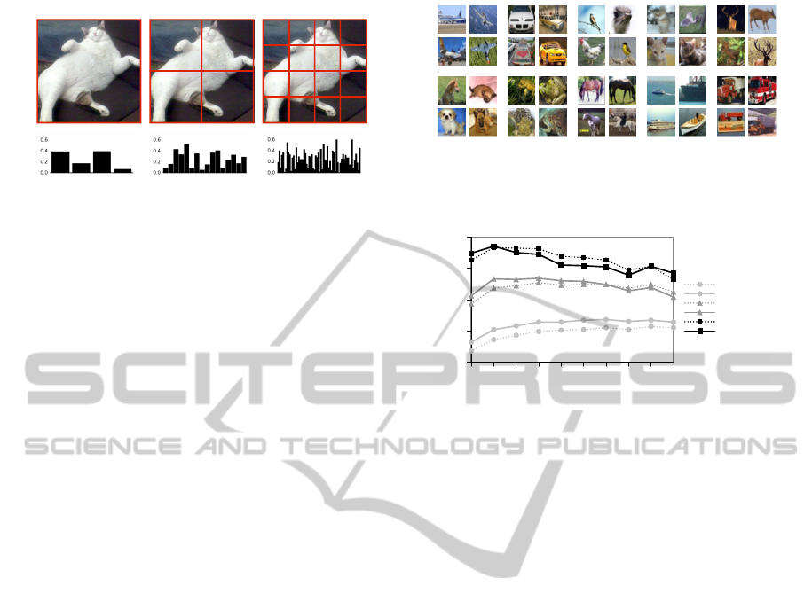
As speciﬁed in Section 1, the dataset used for the

experiments is the CIFAR-10, a very challenging im-

age classiﬁcation dataset that contains 60.000 tiny an-

notated natural images divided into 10 classes, with

6.000 images for each class (Krizhevsky, 2009). The

images, each with a resolution of 32x32 pixels, con-

tain different classes of objects, in particular animals

and vehicles. Figure 3 shows some example images

taken from the CIFAR-10 dataset. In all experiments

we used the training set, composed by 50.000 images,

to learn features and to train the SVM and the test set,

composed by 10.000 images, to test the overall clas-

siﬁcation accuracy. As evaluation metric we used the

percentage overall accuracy (OA), which represents

the number of images correctly classiﬁed on the total

number of images of the test set.

In order to improve the statistical reliability of ac-

curacy values, for each experiment we trained 5 SVM

using 5 disjoint sets of training images and we have

averaged the test results, obtained each one on the

whole test set. We found experimentally that a third

level in the pyramidal histogram increases too much

Figure 3: Four images extracted from each class of the

CIFAR-10 dataset. The classes, from the top-left to the

bottom-right, are: airplane, automobile, bird, cat, deer, dog,

frog, horse, ship and truck.

5 10 15 20 25 30 35 40 45 50

Histogram bins

20%

25%

30%

35%

40%

Overall Accuracy

1 Level (Gray)

1 Level (Color)

2 Levels (Gray)

2 Levels (Color)

3 Levels (Gray)

3 Levels (Color)

Figure 4: Overall accuracy obtained using the PHOG based

classiﬁer, with and without colors.

the size of the training vectors reducing the OA in all

experiments, for this reason we reported results only

for the ﬁrst two levels. All tests reported in the fol-

lowing sections, except those in Section 3.4, were per-

formed using ”grayscale” pixel intensities within re-

ceptive ﬁeld of 6 × 6 pixels with no local brightness

and contrast normalization.

3.1 Standard Classiﬁcation Methods

We now describe the results obtained on the CIFAR-

10 dataset using three standard image classiﬁcation

methods. The ﬁrst method, which we call icon classi-

ﬁer, represents each image as the concatenation of the

intensity values of the pixels. For the color version

of the icon classiﬁer, the feature is formed by con-

catenating for each pixel the value of the three RGB

channels. To control the size of the feature vector

we scaled the image to different sizes, from 1 to 32

pixel square using linear interpolation. The best re-

sult was an OA of 39.5%, obtained using colors and

a 8 pixel squared scaling. Yes, the color is very im-

portant for the classiﬁcation process, giving an im-

provement to the accuracy from 8 to 11%. We then

tested the PHOG method proposed in (Bosch et al.,

2007b), results are shown in Figure 4. We trained the

SVM using a pyramidal histogram of the gradients

computed on both the intensities of the pixels and the

RGB channels. With the PHOG feature the perfor-

mance is always acceptable and grows increasing the

levels of the pyramid. Due to the small size of the

images we could not test the PHOG with 4 levels.

VISAPP2013-InternationalConferenceonComputerVisionTheoryandApplications

598

To exclude that the contribution of the features

learned by the SOM can be due only to the pyramidal

encoding, we performed a test using a pyramidal his-

togram of RGB pixel values. To form the histogram

feature, the RGB space is linear quantized over the

bins of the histograms. Using the aforementioned

method a maximum OA of 38.8% was obtained with

4 bins and a 2 levels histogram. Therefore the pyrami-

dal coding with intensity/RGB feature is not sufﬁcient

to outperform the results obtained with the previously

analyzed icon classiﬁer. The last experiment conﬁrms

that the CIFAR-10 dataset is very hard and we need to

learn ad-hoc features from the dataset itself in order to

achieve results that exceed the 40% accuracy.

3.2 SOM Conﬁguration

In all experiments presented in this work we used

SOM conﬁgured according to the following speciﬁ-

cations. The learning rate α decreases linearly with

the ﬁrst 1000 iterations from 0.1 to 0.01 and for the

next 500 · m iterations from 0.01 to 0.001. These two

learning phases are known in literature as the order-

ing and tuning phases. The parameter σ decreases

linearly from m/2 to 1 during the ordering phase and

from 1 to 0 during the tuning phase. This parame-

ter conﬁguration is widely used and documented in

many works using the SOM model (Kohonen, 1990;

Haykin, 1999). We tried to double, triple and quadru-

ple ordering and tuning iterations, but this did not lead

to any change of more than 0.5% in the classiﬁca-

tion accuracy. Since the number of ordering and tun-

ing iterations corresponds with the number of patches

that the SOM processes and since the total number

of training patches in the CIFAR-10 dataset is much

larger than the number of iterations, it’s important to

present patches to the SOM using a random order.

We conducted ﬁrst experiments using SOMs with

64 to 1024 neurons, doubling at each experiment the

number of neurons. The receptive ﬁeld was set to

6 × 6 pixels. Figure 5 shows overall accuracies in

function of the size of the SOM and the number of

levels in the pyramid. In accordance with the liter-

ature on feature learning, increasing the number of

features leads to improved results, in particular in our

case there is a linear relationship between the square

of the number of neurons involved in the unsuper-

vised learning and the overall classiﬁcation accuracy.

Using the second level of the pyramid, the accuracy

increases from 2.3% to 2.7%. The computational

time required to train a SOM with 512 neurons, us-

ing 4 × 4 pixel patches, was about 20 minutes, or 10

minutes using a 256-neurons SOM. Our implemen-

tation is a single threaded C# code on an Intel(R)

64 128 256 512 1024

SOM size (neurons)

38%

40%

42%

44%

46%

48%

50%

Overall Accuracy

1 Level

2 Levels

Figure 5: Overall accuracy obtained varying the number of

neurons in the SOM and the pyramidal histogram levels.

Xeon(TM) @ 2.66GHz CPU.

3.3 Reducing the Size of the Features

An important property of the SOM model is that

the weights of spatially close neurons correspond to

similar features (Kohonen, 1990). This property is

called topological ordering and is a consequence of

the Equation 2 that forces the weight vector of the

winning neuron and its neighborhood to move toward

the input vector. Exploiting this property we can ar-

bitrarily reduce the number of features used to de-

scribe an image by grouping neighboring neurons in

the same histogram bin. For example, by grouping all

pairs of neighboring neurons it is possible to halve

the size of the ﬁnal feature. Grouping more close

neurons, we can further reduce the size of the fea-

ture and signiﬁcantly speedup the supervised learning

performed by the SVM

We performed some experiments grouping neu-

rons from SOMs with different sizes in order to obtain

several description of images involving histograms

with different number of bins. For example, the rep-

resentation obtained by a 256-neurons SOM was re-

duced in size obtaining histograms with 128, 64 and

32 bins. We also performed a test with a 1024-

neurons SOM where, at the end of the unsupervised

learning process, the neurons were randomly ordered

in order to nullify the effect of the topological order-

ing.

Results reported in Figure 6 clearly shows that the

topological ordering of the SOM allows to efﬁciently

reduce the size of the features without having to re-

train the unsupervised model and without sacriﬁcing

the classiﬁcation quality for more than 1 − 2% accu-

racy. The procedure described above can not be car-

ried out in such a simple way using other not super-

vised methods that do not have the topological order-

ing property, such as the K-means clustering.

In our tests we noticed a 40 − 50% speedup every time

we halved the size of the features used to train the SVM.

UnsupervisedFeatureLearningusingSelf-organizingMaps

599

16 32 64 128 256 512 1024

Number of bins

20%

25%

30%

35%

40%

45%

50%

Overall Accuracy

64 neurons

128 neurons

256 neurons

512 neurons

1024 neurons

1024 neurons (no topology)

Figure 6: Overall accuracy obtained using applying the

topological grouping to reduce the number of bins in the

histogram. In this test we used a 1 Level pyramidal his-

togram.

Gray Color Gray+Norm Color+Norm

Configuration

39%

40%

41%

42%

43%

44%

45%

46%

47%

48%

Overall Accuracy

1 Level

2 Levels

Figure 7: Effect of color, local brightness and contrast nor-

malization for a 64-neurons SOM.

3.4 Improve the Quality of the Features

In this section we report the results obtained using

different receptive ﬁeld sizes, adding the RGB color

information and applying a local brightness and con-

trast normalization to the patches extracted from the

image. Let’s assume that the intensity value of the

pixels varies between 0 and 1, we employed on every

patch extracted from the image a simple normaliza-

tion, subtracting the mean intensity value, dividing

by the standard deviation of its elements and sum-

ming 0.5. Pixel intensities that fall outside the 0 to

1 range after the process are clipped to lie within this

range. Local brightness and contrast normalization

is one of many methods used in feature learning al-

gorithms to improve the quality of the classiﬁcation

results (Coates et al., 2011).

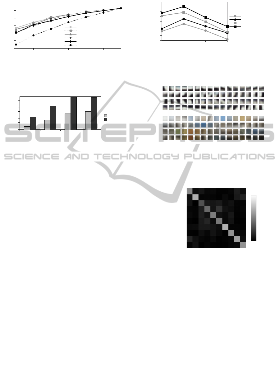
Figure 7 shows the effects of the introduction of

color and local brightness and contrast normalization,

while in Figure 8 we have shown how the classiﬁca-

tion accuracy varies in function of the receptive ﬁeld

size. It is interesting to notice that the use of local

normalization makes the contribution of the color less

important, this fact can be seen also in Figure 9, where

the weights of a 64-neurons SOM, trained with and

without the local normalization are shown.

An OA of 54% was obtained using a 128-neurons

SOM, 4 × 4 pixels receptive ﬁeld, color and local

brightness and contrast normalization, and is compa-

rable with results obtained by (Coates et al., 2011) us-

ing a K-means with a hard pooling feature encoding

2x2 4x4 6x6 8x8

Receptive field size (pixels)

40%

42%

44%

46%

48%

50%

52%

54%

56%

Overall Accuracy

64 neur. (1 level)

128 neur. (1 level)

64 neur. (2 levels)

128 neur. (2 levels)

Figure 8: Effect of receptive ﬁeld size in a 64 and 128-

neurons SOMs, varying the number of pyramid levels. In

this test we used color and local brightness and contrast nor-

malization.

(a)

(b)

Figure 9: Weights plot obtained from a 64-neurons SOM

trained with color 6 × 6 receptive ﬁelds. Effects of training

with (a) and without (b) local contrast and brightness nor-

malization of patches. Notice that the features extracted are

topologically ordered.

Overall Accuracy: 54,14%

100%

20%

40%

60%

80%

(airplane) 1

(automobile) 2

(bird) 3

(cat) 4

(deer) 5

(dog) 6

(frog) 7

(horse) 8

(ship) 9

(truck) 10

Figure 10: Confusion matrix obtained with a 128-neurons

SOM, color, local contrast/brightness normalization and a

4 × 4 pixels receptive ﬁeld.

and a number K of centroids similar to the number of

neurons in our SOM. Figure 10 shows the confusion

matrix for this last experiment.

3.5 Other Datasets

To test the applicability of our method to other

classes of images, we performed a further test on

the very common image classiﬁcation dataset Caltech

101

, containing about 9000 images belonging to 101

classes. The dataset has been split into two sets, 2/3

of the images for training purposes and 1/3 for test-

http://www.vision.caltech.edu/Image Datasets/

Caltech101/

VISAPP2013-InternationalConferenceonComputerVisionTheoryandApplications

600

ing. In order to be processed efﬁciently, each image in

the dataset has been scaled to ﬁt inside a 64 × 64 pix-

els square. We obtained a test accuracy of 87.5% us-

ing a SOM with 1024 neurons, 4 × 4 pixels receptive

ﬁeld, 2 pyramid levels and colors. The same dataset

was processed using the color PHOG feature with 10

bins and 3 levels, obtaining an OA of 74.0%.

4 CONCLUSIONS

In this paper we presented a model that exploits the

Self-Organizing Map (SOM) neural network to learn

features from images without requiring any supervi-

sion. Our experiments performed on the very chal-

lenging CIFAR-10 and on the Caltech 101 datasets

show that the features learned by the SOM and en-

coded using a pyramidal histogram approach signi-

ﬁcatively outperform the classiﬁcation methods based

on raw pixels values and the PHOG feature designed

speciﬁcally for image classiﬁcation. Despite the large

number of images processed in the datasets, the pro-

posed feature learning process is fast and requires few

minutes also using SOMs with hundreds of neurons.

Moreover, employing the presented model it is possi-

ble to control the size of the features used to train the

supervised classiﬁer by grouping close neurons in the

histogram encoding scheme. This property allows to

speed up the learning process without having to repeat

the unsupervised feature learning. Experiments show

that the accuracy of the classiﬁcation can be improved

by applying appropriate normalization and ﬁne tuning

to the receptive ﬁeld. Other normalization methods,

such as whitening (Hyvarinen and Oja, 2000), and

feature encoding schemes, such as hard or soft pool-

ing (Lazebnik et al., 2006; Jarrett et al., 2009), can be

applied to improve the results and will be considered

in future work. An other interesting future develop-

ment is the use of multiple levels of SOM networks

to learn more complex features that can better charac-

terize visual patterns within the images, this approach

has been successfully applied in our previous work

(Vanetti et al., 2012) for the segmentation of complex

textures.

REFERENCES

Bengio, Y., Lamblin, P., Popovici, D., and Larochelle, H.

(2007). Greedy Layer-Wise Training of Deep Net-

works. In Neural Information Processing Systems,

pages 153–160.

Bosch, A., Zisserman, A., and Muoz, X. (2007a). Image

Classiﬁcation using Random Forests and Ferns. In In-

ternational Conference on Computer Vision, pages 1–

Bosch, A., Zisserman, A., and Muoz, X. (2007b). Repre-

senting shape with a spatial pyramid kernel. In Con-

ference on Image and Video Retrieval, pages 401–408.

Coates, A., Lee, H., and Ng, A. Y. (2011). An analysis of

single-layer networks in unsupervised feature learn-

ing. In AISTATS.

Cortes, C. and Vapnik, V. (1995). Support-vector networks.

Machine Learning, 20:273–297.

Csurka, G., Dance, C. R., Fan, L., Willamowski, J., and

Bray, C. (2004). Visual Categorization with Bags of

Keypoints. In European Conference on Computer Vi-

sion.

Gersho, A. and Gray, R. M. (1992). Vector quantization and

signal compression.

Haykin, S. (1999). Neural networks a comprehensive foun-

dation.

Hinton, G. E., Osindero, S., and Teh, Y.-W. (2006). A

Fast Learning Algorithm for Deep Belief Nets. Neural

Computation, 18:1527–1554.

Hinton, G. E. and Salakhutdinov, R. R. (2006). Reduc-

ing the Dimensionality of Data with Neural Networks.

Science, 313:504–507.

Hyvarinen, A. and Oja, E. (2000). Independent component

analysis: algorithms and applications. Neural Net-

works, 13:411–430.

Jarrett, K., Kavukcuoglu, K., Ranzato, M., and LeCun, Y.

(2009). What is the best multi-stage architecture for

object recognition? In International Conference on

Computer Vision, pages 2146–2153.

Kohonen, T. (1990). The self-organizing map. Proceedings

of the IEEE, 78:1464–1480.

Krizhevsky, A. (2009). Learning multiple layers of features

from tiny images. Technical report.

Lazebnik, S., Schmid, C., and Ponce, J. (2006). Beyond

Bags of Features: Spatial Pyramid Matching for Rec-

ognizing Natural Scene Categories. In Computer Vi-

sion and Pattern Recognition, volume 2, pages 2169–

2178.

Le, Q., Ranzato, M., Monga, R., Devin, M., Chen, K., Cor-

rado, G., Dean, J., and Ng, A. (2012). Building high-

level features using large scale unsupervised learning.

In International Conference on Machine Learning.

Lee, H., Battle, A., Raina, R., and Ng, A. Y. (2006). Efﬁ-

cient sparse coding algorithms. In Neural Information

Processing Systems, pages 801–808.

Olshausen, B. A. and Field, D. J. (1996). Emergence of

simple-cell receptive ﬁeld properties by learning a

sparse code for natural images. Nature, 381:607–609.

Raina, R., Madhavan, A., and Ng, A. Y. (2009). Large-scale

deep unsupervised learning using graphics processors.

In International Conference on Machine Learning,

pages 110–880.

Vanetti, M., Gallo, I., and Nodari, A. (2012). Unsuper-

vised self-organizing texture descriptor. In Images:

Fundamentals, Methods and Applications (CompIM-

AGE2012).

UnsupervisedFeatureLearningusingSelf-organizingMaps

601