Accelerated Nonlinear Gaussianization for Feature Extraction
∗
Alexandru Paul Condurache and Alfred Mertins
Institute for Signal Processing, University of Luebeck, Ratzeburger Allee 160, D-23562, Luebeck, Germany
Keywords:
Feature Extraction, Elastic Transform, Gaussianization.
Abstract:
In a multi-class classification setup, the Gaussianization represents a nonlinear feature extraction transform
with the purpose of achieving Gaussian class-conditional densities in the transformed space. The computa-
tional complexity of such a transformation increases with the dimension of the processed feature space in such
a way that only relatively small dimensions can be processed. In this contribution we describe how to reduce
the computational burden with the help of an adaptive grid. Thus, the Gaussianization transform is able to
also handle feature spaces of higher dimensionality, improving upon its practical usability. On both artificially
generated and real-application data, we demonstrate a decrease in computation complexity in comparison to
the standard Gaussianization, while maintaining the effectiveness.
1 INTRODUCTION
Generally, algorithm design is based on some intuitive
insight of the designer into the problem at hand. This
intuition usually comes from the way the designer
perceives the reality surrounding him. In the case of
signal-analysis algorithm design, this sort of intuition
leads more often than wanted to poor solutions, be-
cause it does not correspond to the underlying reality
of the analyzed problem. One major example in this
direction is the intuition of elegant change: change
is not sudden and strong, but rather slow and small.
We have this intuition, because it helps us infer from
some examples what is going to happen next, we thus
know what to expect and get prepared. We are accus-
tomed to reason this way.
We can apply this intuition to a multitude of cases
including observations from a random process. In the
case of classification, for example, this small-change
assumption is equivalent to assuming that the classes
cluster around a center in the feature space. If we de-
cide to model this intuition statistically, then we usu-
ally do this by means of the Gaussian assumption,
like, for example, the Gaussian assumption on the
additive noise term affecting our observations. The
Gaussian assumption tells actually that we expect a
certain thing to happen or some small variations of
that thing, but not large variations, or equivalently,
∗
The authors would like to thank miss Stella Graßhof for
the help she provided with the software implementation of
the Gaussianization transform.
any two consecutive observations from such a distri-
bution are very similar to each other.
Even though the intuition of elegant change is cor-
rect in many cases it is by far not always correct. It
has nevertheless led to the development of a myriad
of methods spanning the entire signal-processing and
analysis spectrum that are optimal only when this in-
tuition is correct, or equivalently under the Gaussian
assumption. These methods are in general charac-
terized as elegant from a mathematical point of view
and intuitive, which has contributed strongly to mak-
ing them ubiquitous, the principal components analy-
sis (PCA) constituting only one of a large number of
possible examples and the linear discriminate analy-
sis (LDA) yet another (Gopinath, 1998).
Besides the relationship between human intuition
and Gaussian assumption, there are also other rea-
sons that make this assumption appealing, like the
Central Limit Theorem, which states that the mean
of n independent identically distributed random vari-
ables, with finite mean and variance, is to the limit
n → ∞ Gaussian (Hogg et al., 2004). Another exam-
ple is related to the statistical properties of this dis-
tribution. These give us the possibility to investigate
complex statistical relationships by relatively simple
mathematical means, like for example independence
relationships considering only moments up to the sec-
ond order (Bishop, 2009).
We address here the question of: what can be done
if the data we analyze does not support the Gaussian
assumption? Our purpose is to transform the analyzed
121
Paul Condurache A. and Mertins A. (2013).
Accelerated Nonlinear Gaussianization for Feature Extraction.
In Proceedings of the 2nd International Conference on Pattern Recognition Applications and Methods, pages 121-126
DOI: 10.5220/0004204701210126
Copyright
c
 SciTePress

data such that it follows a Gaussian distribution, while
at the same time keeping its informative power, such
as to be able to use the familiar Gaussian methods in a
proper way. Our purpose is to achieve gaussianization
for classification purposes. Therefore, in contrast to
other holistic approaches (Chen and Gopinath, 2000),
(Dias et al., 2009), (Saon et al., 2004), (Mezghani-
Marrakchi et al., 2007) that ignore the class-structure
and gaussianize the entire data, we gaussianize the
class-conditional pdfs. We achieve this goal by means
of a transform that modifies the density of the input
data such that this becomes a Gaussian mixture with
the number of modes equal to the number of classes
and the parameters of the modes adapted to the class-
conditional densities.
At this stage it is intuitively clear that the Gaus-
sianization transform should modify the data at a level
that can be achieved only by nonlinear transforma-
tions. A nonlinear transform has virtually complete
control over the input data, the challenge in our case
being to compute the parameters of this transforma-
tion such that the original information available in the
data is still present after applying the transform. Un-
der these circumstances, multiclass Gaussianization
(Condurache and Mertins, 2011) may be achieved
with the help of an elastic transform (Modersitzki,
2004), in a supervised manner, in the sense that it
needs a labeled training set to compute its parame-
ters. The corresponding elastic transform represents
actually a displacement field that shows how should
the data (as present in the feature-space sample from
the training set) be redistributed such as to become
Gaussian. This displacement field is defined over a
grid with a constant distance between grid points. The
difficulty in this case is the computational complex-
ity of the used elastic transform that increases with
the dimension of the input space in such a way that it
becomes prohibitive even for relatively moderate di-
mensions of 15.
With the constant grid, computations are spent for
positions in the feature space where no training data
is present. Assuming that the training space properly
samples the feature space, this is counterproductive.
To decrease the computational burden and thus push
the dimensionality’s upper limit, we introduce here an
adaptive grid for nonlinear Gaussianization. The dis-
tance between grid points in an adaptive grid is vari-
able and the grid is defined in such a way that in the
regions where the data is sparse, the grid is sparse as
well, while in other regions the density of grid points
remains constant as in the fixed grid case. As a con-
sequence the total number of grid points decreases,
while still ensuring a proper link to the feature space.
This paper is structured as follows: in Section 2
we describe adaptive grids and the way we have
adapted them for our gaussianization problem, in Sec-
tion 3 we conduct experiments to show the decrease
in computational burden while still effectively gaus-
sianizing the data, finally in Section 4 we present our
conclusions.
2 ADAPTIVE GRIDS
In the multiclass Gaussianization, the displacement
field that redistributes the data to make it Gaussian
is computed such that the nonparametric estimate of
the available labeled training data is ”morphed“ on
the parametric estimate of the same data. The para-
metric estimate is being computed with the help of a
Gaussian Mixture Model.
The registration between the two pdfs mini-
mizes the sum of squared differences with an elas-
tic constraint, while ignoring probability conserva-
tion (i.e., mass transportation in the sense of Monge-
Kantorovich (Rachev, 1985)) effects to achieve man-
ageable computational complexity.
The displacement filed is discrete, such that the
feature space is divided into a set of intervals. Each
interval is a hyperrectangle with grid points at its cor-
ners.
2.1 A Review of the Elastic Transform
for Multiclass Gaussianization
For the multiclass Gaussianization, we use the train-
ing set to compute the nonparametric pdf estimate of
our data as
p
O
(x) =
1
N · h
m
N
∑
i=1
γ

x − x
i
h

with γ(z) the Gaussian kernel and m the size of the
feature space. The bandwidth parameter h is com-
puted similar to Silverman’s rule of the thumb. Us-
ing the same training set, the parametric pdf estimate
of our data under the assumption of Gaussian class-
conditional distributions is computed as
p
T
(x) =
L
∑
l=1
P
l
· p(x|ω
l
),
where L is the number of classes. P
l
are the a-priori
probabilities of the classes, and p(x|ω
l
) are the multi-
variate Gaussians class-conditional likelihoods (Con-
durache and Mertins, 2011).
Denoting p
O
(x) with O and p
T
(x) with T , the
Gaussianization transform φ : R
d
→ R
d
, with d the di-
mension of the input, modifies O such that it becomes
ICPRAM2013-InternationalConferenceonPatternRecognitionApplicationsandMethods
122

as similar as possible to T. φ = x − u(x) has two parts:
the identity x and the displacement u(x). Given T and
O we look for the displacement u such that
I [u] = D[T, O, u] + αS [u] → min . (1)
where D[T, O; u] is the distance between T and O with
respect to u, S [u] is a regularizing term and α is a
positive real constant. The distance measure D that
we use here is the sum of squared differences
D[T, O;u] =
1
2
kO(φ(x)) − T k
2
L
2
(Ω)
,
with Ω being the region under consideration. As reg-
ularizing term we use the linearized elastic potential
S [u] =
Z
Ω
µ
4
d
∑
j,k=1
(∂
x
j
u
k
+ ∂
x
k
u
j
)
2
+
λ
2
(div u)
2
dx,
with λ and µ being two constants (Modersitzki, 2004).
The solution of the optimization problem (1) is
obtained by numerically solving the corresponding
Euler-Lagrange equations
f = µ4u + (λ + µ)∇div(u) (2)
with f the force related to the distance measure D.
For this purpose we rewrite equation (2) in the form
of the system of differential equations
f = A [u], (3)
with A[u] = µ4u + (λ + µ)∇div(u) a partial differen-
tial operator related to the regularizing term S . To
solve this, a fixed-point iteration scheme is used:
A[u
k+1
](x) = f (x, u
k
(x)), (4)
with A[u
k+1
](x) = A [u
k+1
(x)], x ∈ Ω and k ∈ N.
The transform thus obtained is diffeomorphic. A
displacement field of such an elastic transform is
shown in Figure 2(a).
2.2 Multigrid Methods
Assuming we would like to find the solution to a
generic system of equations in an iterative manner, the
main problem is the initialization. A poor initializa-
tion (i.e., the initial solution is very far from the true
one) leads to a large number of iterations that need
to be computed to reach the vicinity of the true so-
lution. Thus, to speed up such algorithms we need a
good initialization. Multigrid considerations (Wessel-
ing, 1992), (Trottenberg et al., 2001) are instrumental
on this path.
Within the context of differential equations, the
multigrid approach comes naturally when considering
discrete approximations. Discrete approximations of
differential equations are either used to approximate
the solution numerically with the help of a computer
or they arise naturally for example in the field of digi-
tal signal processing, as in the case of image registra-
tion or our nonlinear Gaussianization.
In our case, when we need to solve equation (3)
we would first find a solution to a reduced system of
equations, corresponding to a coarse grid. In com-
parison to a dense grid, the coarse grid is obtained
by disregarding some points and the reduced system
of equations is obtained by eliminating the equations
corresponding to the disregarded points. After com-
puting the coarse-grid solution, we would extrapolate
this reduced solution to the entire system and use this
as initialization for the iterative scheme (4). The dif-
ficulty with this approach is related to the frequency
characteristics of the error, as high-frequency errors
cannot be well approximated on a coarser grid (Hack-
busch, 1993).
2.3 Adaptive Multigrid Methods for
Nonlinear Gaussianization
Adaptive grids have been used already to decrease the
computation burden but also to increase the accuracy
of multigrid methods applied to the solving of PDEs.
The core idea is to spend computational power only
where it is needed, i.e, around the areas of interest,
where the change occurs. There are two main ways to
implement this idea (Trottenberg et al., 2001), in the
form of static (predefined) adaptive grids and dynamic
(self-adaptive) adaptive grids. In the former case the
structure of the grid is defined before the computa-
tion starts and in the latter case, the grid modifies its
structure during the computation.
Multigrid (including adaptive grid) numerical
methods represent efficient and general ways to solve
the systems of equations arising in our Gaussianiza-
tion, i.e., at each step of the fixed point iteration
scheme in equation (4). We have used them as inspi-
ration for an accelerated Gaussianization that works
with an adaptive grid. The idea that we follow here
is simple: we observe that in our training set, the data
points are not uniformly distributed over Ω, therefore,
instead of computing the displacement field over a
fixed grid, we may want to compute it over a vari-
able grid that is dense where the data is dense and
sparse where the data is sparse. The grid size δ of
the standard Gaussianization, empirically defined as
δ = log
10
(tr(Σ)), with Σ the covariance matrix of the
training data, becomes now the lower bound of an
adaptive grid. As in the case of the standard Gaussian-
ization, the maximal span of the data-centered grid is
two times the standard deviation of the training sam-
AcceleratedNonlinearGaussianizationforFeatureExtraction
123

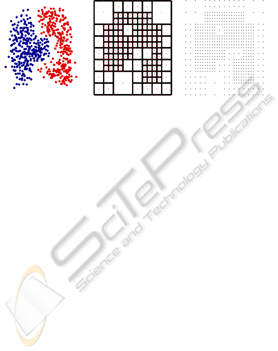
Figure 1: Shown here are: first the original non-Gaussian data (the class affiliation is color coded), then the adaptive grid
as red dots with the subregions R
i
, drawn with black lines (the smallest subregions are not drawn for display purposes) and
finally the adaptive grid.
ple in each direction.
For our Gaussianization purposes we introduce
here a predefined adaptive grid. As a consequence the
total number of grid points decreases, while still en-
suring a proper link to the feature space. To construct
the adaptive grid, we determine its granularity in non-
overlapping hypersquare-sub-regions of Ω (see Fig-
ure 1). The adaptive grid is used in the fixed point iter-
ation (4). The iteration is conducted first at the coars-
est grid, and then hypersquare-wise at finer grids, us-
ing as initialization the extrapolated result from the
previous coarser grid. At each iteration the corre-
sponding system of equations is solved with the Con-
jugate Gradient (CG) method. An accelerated Gaus-
sianization displacement field is shown in Figure 2(b).
There is no standard solution for the problem of
defining an adaptive grid in this context. We make
here use of a heuristic derived from the field of im-
age segmentation into two classes: object and back-
ground. Our heuristic stems from the region splitting
image-segmentation algorithm (Gonzales and Woods,
2008). This is a region-based procedure that makes
use of a homogeneity criterion H(R) to find out if a
certain region R
i
of the input image is part of the ob-
ject or of the background. As a result, the image I is
divided into non-overlapping regions R
i
, i = 1 . . . , N,
such that:
N
[
i=1
R
i
= I, ∀i : R
i
⊆ I, ∀i 6= j : R
i
∩ R
j
= 0.
Each region satisfies H(R
i
). For a 2D image, region-
splitting procedure begins by considering the entire
image one region. If H(R) is not fulfilled, then R is
divided into four new regions, by halving each side
of the initial region. This division step is repeated as
long as H(R
i
) = f alse. We obtain thus a data struc-
ture similar to a quadtree.
To implement the variable grid, we adapt the
region-splitting procedure to our purposes. The fore-
ground is there where the data is concentrated, while
the background is there where the data is sparse.
Therefore, our homogeneity criterion has to measure
how sparse the data is in a region, and to do so we
define H(R
i
) as
H(R
i
) :
(
true, if
k
R
i
k
0
≤ τ
false, otherwise
where
k
R
i
k
0
is the number of data points in R
i
and τ
is a threshold.
τ is defined with the help of δ, the size of the static
transform grid, as the maximum of the number of data
points that can be found in a hypercube of side δ. We
use this definition such as to ensure that at its finest
granularity, the adaptive grid is similar to the static
grid and thus we achieve a true reduction of the num-
ber of grid points in comparison to the standard Gaus-
sianization. The computation of the variable grid is
illustrated in Figure 1.
The region-splitting procedure establishes the size
of a hypersquare region such that each region has a
similar number of data points in it. Therefore, a re-
gion is large where the data is sparse and small where
the data is dense. After dividing Ω with the help of
the region-splitting procedure, for each region R
i
we
need to define the grid-size δ
i
. Clearly, the grid size is
related to the size of the respective region and we set
δ
i
, to be the side of the corresponding hypersquare.
Therefore, similar to the region itself, δ
i
will be large
where the data is sparse and thus we will have there
a small number of grid points. Conversely, δ
i
will be
small where the data is dense and in these regions we
will have a large number of grid points.
ICPRAM2013-InternationalConferenceonPatternRecognitionApplicationsandMethods
124

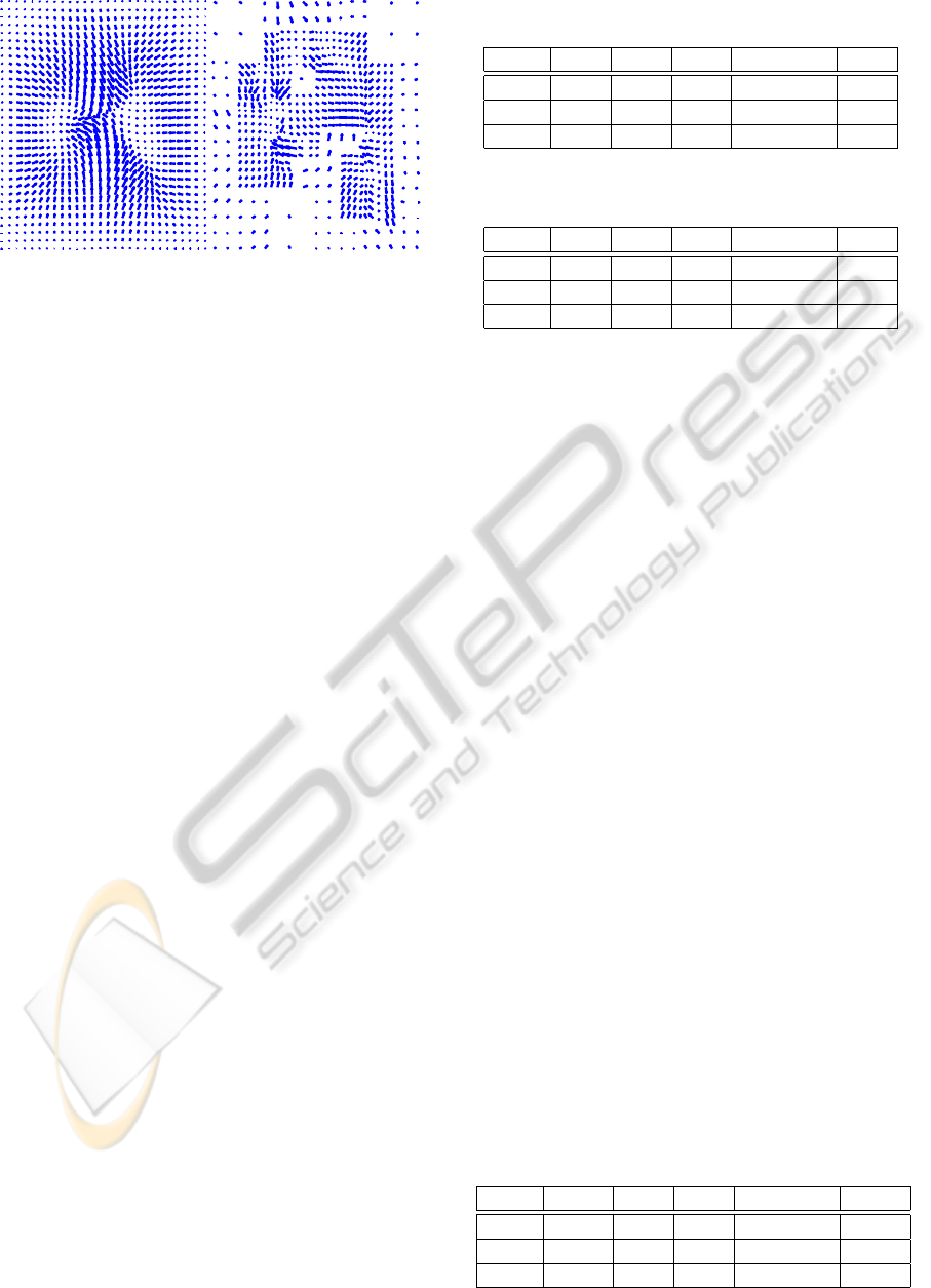
(a) (b)
Figure 2: Displacement field for the standard, static-grid
transform (a) and for the accelerated, adaptive-grid trans-
form (b), for the two-class input data from Figure 1.
3 EXPERIMENTS AND
DISCUSSION
We have successfully tested the multiclass Gaussian-
ization on both synthetic and real data. The synthetic
data was of two types: linearly separable data and
nonlinearly separable data. Each time we have gen-
erated 800 data points. The real data was Fischer’s
”iris” dataset (Bezdek et al., 1999), with three classes
and 150 data points, which is not separable. The syn-
thetic data was 2D and the real data 4D. The Gaus-
sianization was computed on a training set made of
50% of the respective data set. The test consisted on
applying various Gaussian density-related classifiers
to the data before (O) and after both standard (G) and
accelerated Gaussianization (accG). After Gaussian-
ization the results improved, in the sense that less er-
rors were made on the test set. These classifiers were:
(i) a white Gaussian Bayesian classifier computed un-
der the assumption of equal, unit class covariance ma-
trices (W), (ii) a linear Gaussian Bayesian classifier
computed under the assumption of equal class covari-
ance matrices (L), (iii) a nonlinear Gaussian Bayesian
classifier (nL), (iv) a support vector machine with a
Radial Basis Function kernel (SVM) – with the num-
ber of support vectors (sv) in the brackets – and (v) a
linear perceptron (P). The results have been computed
on a test set made of the remaining 50% of each data
set. We have conducted the same experiments with
the adaptive-grid Gaussianization and obtained the
largely similar results, shown in Tables 1, 2 and 3. To
investigate the decrease in computational complexity
of the Gaussianization when using the adaptive grid,
we have computed the size of each grid (i.e., number
of grid points), for each of the tested datasets: linearly
separable (2D-lin.), nonlinearly separable (2D-nlin.)
and the ”iris” dataset (4D). The results are shown in
Table 1: Error rates (%) of various classifiers before and
after Gaussianization on the linearly separable dataset.
W L nL SVM (sv) P
O 1.75 0.75 0.75 0 (15) 0.25
G 0.25 0 0 0 (11) 0
accG 0.25 0 0 0 (12) 0
Table 2: Error rates (%) of various classifiers before and
after Gaussianization on the nonlinearly separable dataset.
W L nL SVM (sv) P
O 5.25 4.25 4.25 1.25 (17) 3.75
G 2.25 1.75 1.75 0.25 (12) 1.75
accG 2.75 2 2 0.25 (14) 1.75
Table 4. We have measured the time needed for each
type of Gaussianization under MATLAB on a dual-
core Opteron 8222 machine at 3GHz with 16GB of
RAM in each scenario. The results show a decrease in
computational time of at most 10%, even if the num-
ber of grid points is halved. The computation of the
displacement field of the standard Gaussianization for
the 4D ”iris“ dataset takes approximatively two min-
utes.
4 CONCLUSIONS, SUMMARY
AND OUTLOOK
The multiclass Gaussianization, as proposed in (Con-
durache and Mertins, 2011), is a novel type of feature
extraction transform. In comparison to other feature
extraction methods it does not have as purpose dimen-
sionality reduction or improved separability, but the
modification of the density of the input data, such that
each class is Gauss distributed. State-of-the-art multi-
class Gaussianization is computationally demanding,
which represents an obstacle in the practical deploy-
ment of such methods, even if for a certain classifi-
cation problem it has to be computed only once, dur-
ing the training phase. Therefore, in this contribu-
tion we have proposed and demonstrated a method to
decrease the computational burden of the multiclass
Gaussianization.
As in the case of the standard Gaussianization, the
accelerated Gaussianization that we have introduced
Table 3: Error rates (%) of various classifiers before and
after Gaussianization on the ”iris” dataset.
W L nL SVM (sv) P
O 8 2.66 2.67 1.33 (20) 10.66
G 10.66 1.33 0 0 (17) 14.66
accG 8 1.33 0 0 (15) 8
AcceleratedNonlinearGaussianizationforFeatureExtraction
125

Table 4: Grid complexity for various datasets.
Dimension Type Grid size
2D-lin.
std. 1056
acc. 563
2D-nlin.
std. 924
acc. 589
4D
std. 2520
acc. 2157
effectively makes the data more Gaussian, as shown
by the improved performance of Gauss-related classi-
fiers in the transformed space. We believe that the
small increases of the error rate on the nonlinearly
separable data set are due to the fact that in the re-
gions where the adaptive grid is sparse, the displace-
ment vectors of the nonlinear transform are larger –
which follows from the very way the transform is
computed. Test-set points falling in regions of the
feature space covered by a coarse section of the adap-
tive grid will tend to travel further away, potentially
over the linear separation surface, but they do so in
a grouped manner, such that in the case of the SVM,
new support vectors placed there lead to the group be-
ing correctly classified. Still the number of support
vectors is smaller than for the original data, as it may
be observed in Table 2. Conversely the same behavior
works to our advantage on the ”iris” dataset.
The main purpose of the accelerated Gaussian-
ization is to reduce the training time (i.e., the time
needed to compute the parameters of the elastic trans-
form), so that to be able to apply the Gaussianization
to features spaces of higher dimension. The accel-
erated Gaussianization works by reducing the size of
the grid where the elastic transform is computed and
offering better initialization locally for the conjugate-
gradient solver. On the other hand, the parameters
of several gird points (i.e, those also present on the
coarser previous grid) are recomputed each time the
grid turns finer in the respective region. Furthermore,
with the adaptive grid some time is spent during the
computation of the transform with the generation of
the adaptive grid and then with the management of the
adaptive grid. Therefore, the time does not decrease
linearly with the number of grid points. Nevertheless,
as a whole, we are able to reduce the time needed
to train the Gaussianization, because, even if some
grid points are recomputed several times, as a total, a
smaller number of equations needs to be solved. Fur-
thermore, the CG solver coverages in a smaller num-
ber of steps due to the improved initialization.
The process can be speed up even further if we
use faster solvers than the CG. A last resort solution
to achieve a significant reduction in complexity for
problems of very large size would be to reduce the
dimensionality of the feature space before Gaussian-
ization. It remains to be investigated if this is a viable
solution and how should it be implemented precisely.
We have introduced and successfully tested an
adaptive grid setup to speed up the computation of the
parameters of the nonlinear multi-class Gaussianiza-
tion transform. The adaptive grid is computed so that
to ensure that the same number of training-set vec-
tors is present in each hyperrectangle with grid-points
at its corners. The adaptive grid Gaussianization ef-
fectively makes the input data more Gaussian, while
reducing the computational complexity.
REFERENCES
Bezdek, J., Keller, J., Krishnapuram, R., Kuncheva, L., and
Pal, N. (1999). Will the real iris data please stand up?
IEEE Trans. on Fuzzy Systems, 7(3):368–369.
Bishop, C. M. (2009). Pattern recognition and machine
learning. Information Science and Statistics. Springer.
Chen, S. and Gopinath, R. (2000). Gaussianization. In Proc.
of NIPS, Denver, USA.
Condurache, A. P. and Mertins, A. (2011). Elastic-
transform based multiclass gaussianization. IEEE Sig-
nal Processing Letters, 18(8):482–485.
Dias, T. M., Attux, R., Romano, J. M., and Suyama, R.
(2009). Blind source separation of post-nonlinear
mixtures using evolutionary computation and gaus-
sianization. In Proc. of ICA, pages 235–242. Springer.
Gonzales, R. C. and Woods, R. E. (2008). Digital image
processing (Third edition). Pearson Education.
Gopinath, R. A. (1998). Maximum likelihood modeling
with gaussian distributions for classification. In Proc.
of ICASSP, pages 661–664, Seattle, U.S.A.
Hackbusch, W. (1993). Iterative solution of large sparse
systems of equations. Springer-Verlag (New York).
Hogg, R., Craig, A., and McKean, J. (2004). Introduction
to mathematical statistics. Prentice Hall, 6 edition.
Mezghani-Marrakchi, I., Mah, G., Jadane-Sadane, M.,
Djaziri-Larbi, S., and Turki-Hadj-Allouane, M.
(2007). ”gaussianization” method for identification
of memoryless nonlinear audio systems. In Proc. of
EUSIPCO, pages 2316 – 2320.
Modersitzki, J. (2004). Numerical methods for image reg-
istration. Oxford university press.
Rachev, S. T. (1985). The Monge-Kantorovich mass trans-
ference problem and its stochastic applications. SIAM
Theory of Probability and its Applications, 29(4):647
– 676.
Saon, G., Dharanipragada, S., and Povey, D. (2004). Fea-
ture space gaussianization. In Proc. of ICASSP, pages
I – 329–332.
Trottenberg, U., Oosterlee, C. W., and Schller, A. (2001).
Multigrid. Academic Press.
Wesseling, P. (1992). An introduction to multigrid methods.
John Wiley & Sons.
ICPRAM2013-InternationalConferenceonPatternRecognitionApplicationsandMethods
126