Improved Boosting Performance by Exclusion

of Ambiguous Positive Examples

Miroslav Kobetski and Josephine Sullivan

Computer Vision and Active Perception, KTH, Stockholm 10800, Sweden

Keywords:

Boosting, Image Classiﬁcation, Algorithm Evaluation, Dataset Pruning, VOC2007.

Abstract:

In visual object class recognition it is difﬁcult to densely sample the set of positive examples. Therefore,

frequently there will be areas of the feature space that are sparsely populated, in which uncommon examples

are hard to disambiguate from surrounding negatives without overﬁtting. Boosting in particular struggles to

learn optimal decision boundaries in the presence of such hard and ambiguous examples. We propose a two-

pass dataset pruning method for identifying ambiguous examples and subjecting them to an exclusion function,

in order to obtain more optimal decision boundaries for existing boosting algorithms. We also provide an

experimental comparison of different boosting algorithms on the VOC2007 dataset, training them with and

without our proposed extension. Using our exclusion extension improves the performance of all the tested

boosting algorithms except TangentBoost, without adding any additional test-time cost. In our experiments

LogitBoost performs best overall and is also signiﬁcantly improved by our extension. Our results also suggest

that outlier exclusion is complementary to positive jittering and hard negative mining.

1 INTRODUCTION

Recent efforts to improve image classiﬁcation perfor-

mance have focused on designing new discrimina-

tive features and machine learning methods. How-

ever, some of the performance gains of many well-

established methods are due to dataset augmentation

such as hard negative mining, positive mirroring and

jittering (Felzenszwalb et al., 2010; Dalal and Triggs,

2005; Laptev, 2009; Kumar et al., 2009). These data-

bootstrapping techniques aim at augmenting sparsely

populated regions of the dataset to allow any learn-

ing method to describe the class distributions more

accurately, and they have become standard tools for

achieving state-of-the-art performance for classiﬁca-

tion and detection tasks. In this paper we revisit the

dataset augmentation idea, arguing and showing that

pruning the positive training set by excluding hard-to-

learn examples can improve performance for outlier-

sensitive algorithms such as boosting.

We focus on the boosting framework and propose

a method to identify and exclude positive examples

that a classiﬁer is unable to learn, to make better use

of the available training data rather than expanding it.

We refer to the non-learnable examples as outliers and

we wish to be clear that these examples are not label

noise (such as has been studied in (Long and Serve-

dio, 2008; Masnadi-shirazi and Vasconcelos, 2008;

Leistner et al., 2009)), but rather examples that with a

given feature and learner combination are ambiguous

and too difﬁcult to learn.

One of the main problems with most boosting

methods is their sensitivity to outliers such as atypical

examples and label noise (Bauer and Kohavi, 1999;

Dietterich, 2000; Freund and Science, 2009; Long

and Servedio, 2008). Some algorithms have tried to

deal with this problem explicitly (Freund, 1999; Fre-

und and Science, 2009; Masnadi-Shirazi et al., 2010;

Grove and Schuurmans, 1998; Warmuth et al., 2008;

Masnadi-shirazi and Vasconcelos, 2008), while oth-

ers, such as LogitBoost (Friedman et al., 2000) are

less sensitive due to their softer loss function.

The boosting methods with aggressive loss func-

tions give outliers high weight when ﬁtting the weak

learner, and therefore potentially work poorly in the

presence of outliers. Softer loss function as seen in the

robust algorithms can on the other hand result in low

weights for all examples far from the margin, regard-

less if they are noisy outliers or just data to which the

current classiﬁer has not yet been able to ﬁt. This can

be counter-productive in cases of hard inliers, which

is illustrated in ﬁgure 2(a). Another problem that soft

loss functions are not able to solve is that outliers are

still able to affect the weak learners during the early

Kobetski M. and Sullivan J. (2013).

Improved Boosting Performance by Exclusion of Ambiguous Positive Examples.

In Proceedings of the 2nd International Conference on Pattern Recognition Applications and Methods, pages 11-21

DOI: 10.5220/0004204400110021

 SciTePress

(a) Chair class

(b) Bottle class

Figure 1: Examples of outliers and inliers. The top rows

of (a) and (b) show outliers while the bottom rows show

inliers. We focus on how to detect the outliers and how their

omission from training improves test results. The images

are from the VOC2007 dataset.

stages of the training, which due to the greedy nature

of boosting can only be undone later on by increasing

the complexity of the ﬁnal classiﬁer.

In this paper we provide an explicit analysis on

how various boosting methods relate to examples via

their weight functions and we argue that a distinct

separation in the handling of inliers and outliers can

help solve these problems that current robust boosting

algorithms are facing.

Following this analysis we propose our two pass

boosting algorithm extension, that explicitly handles

learnable and non-learnable examples differently. We

deﬁne outliers as examples that are too hard-to-learn

for a given feature and weak learner set, and identify

them based on their classiﬁcation score after a ﬁrst

training round. A second round of training is per-

formed, where the outliers are subjected to a much

softer loss function and are therefore not allowed to

interfere with the learning of the easier examples, in

order to ﬁnd a better optimum. This boosting algo-

rithm extension consistently gives better test perfor-

mance, with zero extra test-time costs at the expense

of increased training time. Some examples of found

inliers and outliers can be seen in ﬁgure 1.

1.1 Relation to Bootstrapping Methods

To further motivate our data-centric approach to

learning, we illustrate the problems that different

dataset augmentation techniques address. In regions

where the positive training examples are dense and

the negatives are existent but sparse, hard negative

mining might improve the chances of ﬁnding the op-

timal decision boundary. In regions where positives

are sparse and negatives existent, jittering and mirror-

ing might have some effect, but the proper analogue

to hard negative mining is practically much harder,

since positive examples need to be labelled. At some

scale this can be done by active learning (Vijaya-

narasimhan, 2011), where labelling is done iteratively

on selected examples. Our approach tries to handle

the regions where positives are sparse but additional

hard positive mining is not possible, either due to lim-

ited resources or because all possible positive min-

ing has already been done. We address this problem

by restricting hard-to-learn positives from dominat-

ing the training with their increasingly high weights

by excluding them from the training.

Our algorithm can be considered as dataset prun-

ing and makes us face the philosophical question of

more data vs. better data. It has been shown that in

cases where huge labelled datasets are available, even

simple learning methods perform very well (Shotton

et al., 2011; Torralba et al., 2008; Hays and Efros,

2007). We address the opposite case, where a huge

accurately labelled data set cannot be obtained - a

common scenario both in academic and industrial

computer vision.

1.2 Contributions

We propose a two-pass boosting extension algorithm,

suggested by a weight-centric theoretical analysis of

how different boosting algorithms respond to outliers.

We also demonstrate that it is important to distin-

guish between ”hard-to-learn” examples and ”non-

learnable” outliers in vision as examples easily iden-

tiﬁed as positive by humans could be non-learnable

given a feature and weak-learner set, and demonstrate

that the different classes in VOC2007 dataset indeed

have different fractions of hard-to-learn examples us-

ing HOG as base feature. Finally we provide exten-

sive experimental comparison of different boosting al-

gorithms on real computer vision data and perform

experiments using dataset augmentation techniques,

showing that our method is complementary to jitter-

ing and hard negative mining.

2 RELATION TO PREVIOUS

WORK

As previously mentioned AdaBoost has been shown

ICPRAM2013-InternationalConferenceonPatternRecognitionApplicationsandMethods

to be sensitive to noise (Bauer and Kohavi, 1999; Di-

etterich, 2000). Other popular boosting algorithms

such as LogitBoost or GentleBoost (Friedman et al.,

2000) have softer loss functions or optimization meth-

ods and can perform better in the presence of noise in

the training data, but they have not been speciﬁcally

designed to handle this problem. It has been argued

that no convex-loss boosting algorithm is able to cope

with random label noise (Long and Servedio, 2008).

This is however not the problem we want to address,

as we focus on naturally occurring outliers and am-

biguous examples, which is a signiﬁcant and interest-

ing problem in object detection today.

BrownBoost (Freund, 1999) and RobustBoost

(Freund and Science, 2009) are adaptive extensions of

the Boost-By-Majority Algorithm (Freund, 1995) and

have non-convex loss functions. Intuitively these al-

gorithms “give up” on hard examples and this allows

them to be less affected by erroneous examples.

Regularized LPBoost, SoftBoost and regularized

AdaBoost (Warmuth et al., 2008; R

atsch et al., 2001)

regularize boosting to avoid overﬁtting to highly

noisy data. These methods add the concept of soft

margin to boosting by adding slack variables in a sim-

ilar fashion to soft-margin SVMs, and this decreases

the inﬂuence of outliers. Conceptually these methods

bear some similarity to ours as the slack variables re-

duce the inﬂuence of examples on the wrong side of

the margin, and they deﬁne an upper bound on the

fraction ν of misclassiﬁed examples, which is com-

parable to the fraction of the dataset excluded in the

second phase of training.

There is recent work on robust boosting where

new semi-convex loss functions are derived based on

probability elicitation (Masnadi-Shirazi et al., 2010;

Masnadi-shirazi and Vasconcelos, 2008; Leistner

et al., 2009). These methods have shown potential for

high-noise problems such as tracking, scene recog-

nition and artiﬁcial label noise. But they have not

been extensively compared to the common outlier-

sensitive algorithms on low-noise problems, such as

object classiﬁcation, where the existing outliers are

ambiguous or uncommon examples, rather than ac-

tual label errors.

In all the mentioned robust boosting algorithms

the outliers are estimated and excluded on the ﬂy and

these outliers are therefore able to affect the training

in the early rounds. Also, as can be seen in ﬁgure 2,

these algorithms can treat uncommon non-outliers as

conservatively as actual outliers, resulting in subopti-

mal decision boundaries.

Reducing overﬁtting by pruning the training set

has been studied previously (Vezhnevets and Bari-

nova, 2007; Angelova et al., 2005) but improved re-

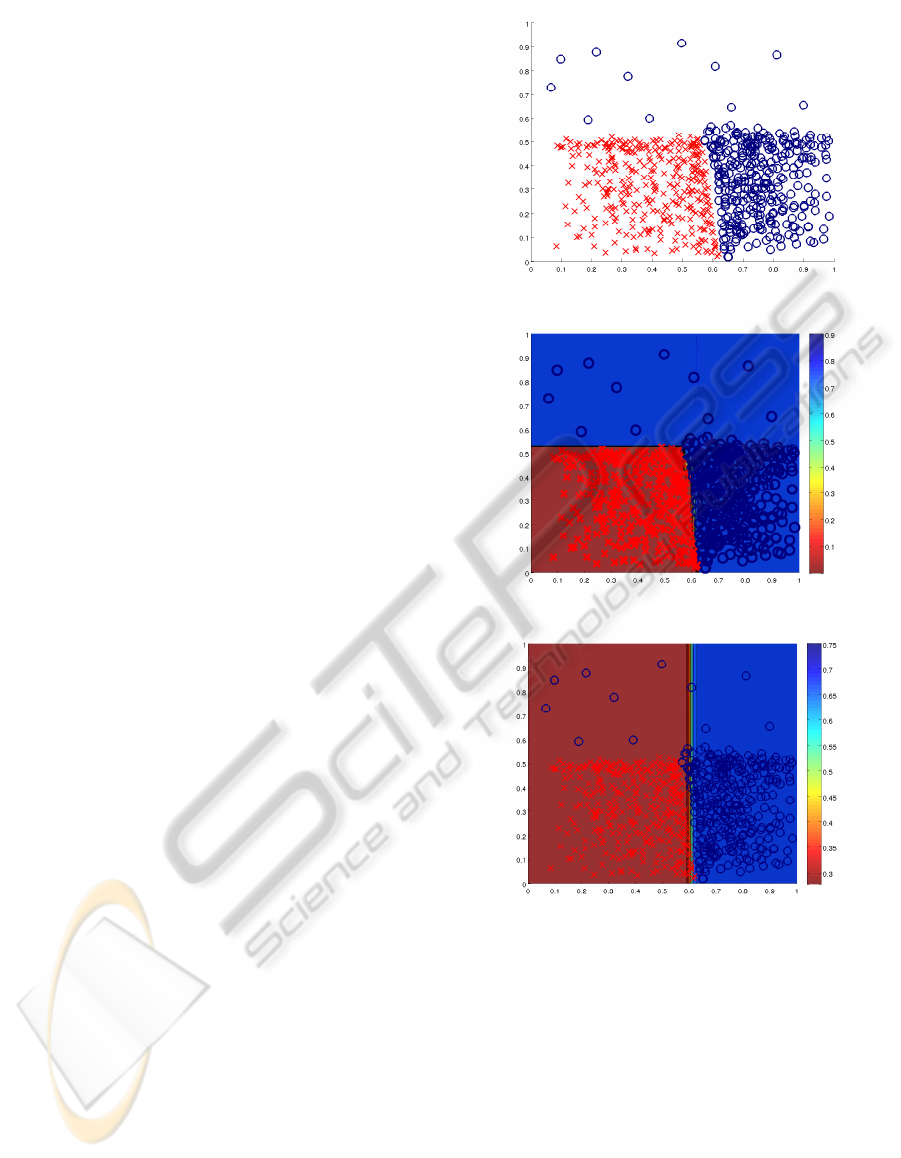
(a) Toy example without outliers

(b) Learnt AdaBoost classiﬁer

Figure 2: Example with hard inliers. This toy problem

shows how less dense, but learnable examples do not con-

tribute to the decision boundary when learned using Robust-

Boost. The colour coding represents estimated probability

p(y = 1|x). (Best viewed in colour.)

sults have mostly been seen in experiments where

training sets include artiﬁcial label noise. (Vezhn-

evets and Barinova, 2007) is the only method that we

have found where pruning improves performance on a

“clean” dataset. (Vezhnevets and Barinova, 2007) use

an approach very similar to ours, detecting hard-to-

learn examples, then removing those examples from

training. The base algorithm to which (Vezhnevets

and Barinova, 2007) apply dataset pruning is Ad-

ImprovedBoostingPerformancebyExclusionofAmbiguousPositiveExamples

aBoost, which we show is the most noise-sensitive

boosting algorithm and not the one that should be

used for image classiﬁcation. When comparing to a

more robust boosting algorithm the robust non-pruned

algorithm (MadaBoost) that they use and the pruned

AdaBoost turn out to be roughly equivalent. The re-

sults show 5-4 in wins and 15.109% vs. 15.044%

in average test error when using 100 weak learn-

ers. To get an improvement using their method they

have to push the learning beyond the limit of over-

ﬁtting by training a huge number of weak learners

(13-300 weak learners per available data dimension).

We propose a similar but more direct approach that

improves results for both robust and non-robust algo-

rithms, while still using a reasonable number of weak

learners.

Also it is important to note that vision data is typ-

ically very high-dimensional and boosting therefore

also acts as feature selection - learning much fewer

weak learners than available dimensions. Due to the

mentioned differences between vision and machine

learning datasets, it is not easy to directly transfer

the results from (Vezhnevets and Barinova, 2007) to

vision without experimental validation. Our experi-

ments on the VOC2007 dataset verify that exclusion

of ambiguous examples, as seen in our paper and

in (Vezhnevets and Barinova, 2007), translates well

to the high-dimensional problems found in computer

vision. We also compare a number of well-known

boosting algorithms using typical vision data, some-

thing that we have not seen previously.

A different but related topic that deals with label

ambiguity is Multiple Instance Learning (MIL). Viola

et al. (Viola and Platt, 2006) suggest a boosting ap-

proach to the MIL problem, applying their solution to

train an object detector with highly unaligned training

data.

Our idea is also conceptually similar to a sim-

pliﬁed version of self-paced learning (Kumar and

Packer, 2010). We treat the hard and easy positives

separately and do not let the hard examples dominate

the easy ones in the search for the optimal decision

boundary. This can seen as a heavily quantized ver-

sion of presenting the examples to the learning algo-

rithm in the order of their difﬁculty.

3 BOOSTING THEORY

Boosted strong classiﬁers have the form H

(x) =

∑

h(x;β

), where h(x) is a weak learner, with

multiplier α

and parameters β

. To learn such a

classiﬁer one wishes to minimize the average loss

∑

j=1

L(H(x

),y

) over the N input data points

) where each data label y

∈ {−1, 1}. Learn-

ing the classiﬁer that minimizes the average loss by

an exhaustive search is infeasible, so boosting al-

gorithms do this in a greedy stepwise fashion. At

each iteration the strong classiﬁer is extended with the

weak learner that minimizes the loss given the already

learned strong classiﬁer

∗

,β

∗

= argmin

α,β

∑

j=1

L(H

) + αh(x

;β),y

(1)

Equation 1 is solved by weighting the importance

of the input data by a weight function w(x, y) when

learning α and β. This w(x

) represents how

poorly the current classiﬁer H

) is able to classify

example j.

Different boosting algorithms have different

losses and optimizations procedures, but the key

mechanism to their behaviour and handling of outliers

is the weight function w(x, y). For this reason we be-

lieve that analyzing the weight functions of different

losses give an insight to how different boosting algo-

rithms behave in the presence of hard and ambigu-

ous examples. So in order to compare a number of

boosting algorithms in a consistent framework we re-

derive w(x, y) for each of the algorithms by following

the GradientBoost approach (Friedman, 2001; Mason

et al., 1999).

The GradientBoost approach view boosting as a

gradient based optimization of the loss in function

space. According to the GradientBoost framework a

boosting algorithm can be constructed from any dif-

ferentiable loss function, where each iteration is a

combination of a least squares ﬁtting of a weak re-

gressor h(x) to a target w(x,y)

∗

= argmin

∑

(w(x

) − h(x

;β))

, (2)

and a line search α = argmin

(L(H(x) + αh(x;β))) to

obtain α. The loss function is derived with respect to

the current margin v(x, y) = yH(x) to obtain the neg-

ative target function

w(x,y) = −

∂L(x,y)

∂v(x,y)

. (3)

Equation 2 can then be interpreted as ﬁnding the weak

learner that points in the direction of the steepest gra-

dient of the loss, given the data.

3.1 Convex-loss Boosting Algorithms

3.1.1 Exponential Loss Boosting

AdaBoost and GentleBoost (Freund and Schapire,

1995; Friedman et al., 2000) are the most notable al-

ICPRAM2013-InternationalConferenceonPatternRecognitionApplicationsandMethods

gorithms with the exponential loss

(x,y) = exp(−v(x, y)). (4)

AdaBoost uses weak classiﬁers for h(x) rather

than regressors and directly solves for α, while Gen-

tleBoost employs Newton-step optimization for the

expected loss. In the original algorithms w(x,y) is

exponential and comes in via the weighted ﬁtting of

h(x), but we obtain

(x,y) = exp(−v(x, y)), (5)

from the GradientBoost approach to align all ana-

lyzed loss functions in the same framework. w

(x,y)

has a slightly different meaning than the weight func-

tion of the original algorithms since it is the tar-

get of a non-weighted ﬁt, rather than the weight of

a weighted ﬁt. However, its interpretation is the

same - the importance function by which an exam-

ple is weighted for the training of the weak learner

h(x). Also, it should be noted that we have omit-

ted implementation-dependent normalization of the

weight function.

3.1.2 Binomial Log-likelihood Boosting

LogitBoost is a boosting algorithm that uses Newton

stepping to minimize the expected value of the nega-

tive binomial log-likelihood

(x,y) = log(1 + exp(−2v(x,y))). (6)

This is potentially more resistant to outliers than Ad-

aBoost or GentleBoost as the binomial log-likelihood

is a much softer loss function than the exponential one

(Friedman et al., 2000).

Since the original LogitBoost optimizes this loss

with a series of Newton steps, the actual importance

of an example is distributed between a weight func-

tion for the weighted regression and a target for the

regression - both varying with the margin of the exam-

ple. We derive w(x,y) by applying the GradientBoost

approach to the binomial log-likelihood loss function

to collect the example weight in one function

(x,y) =

1 + exp (v(x,y))

. (7)

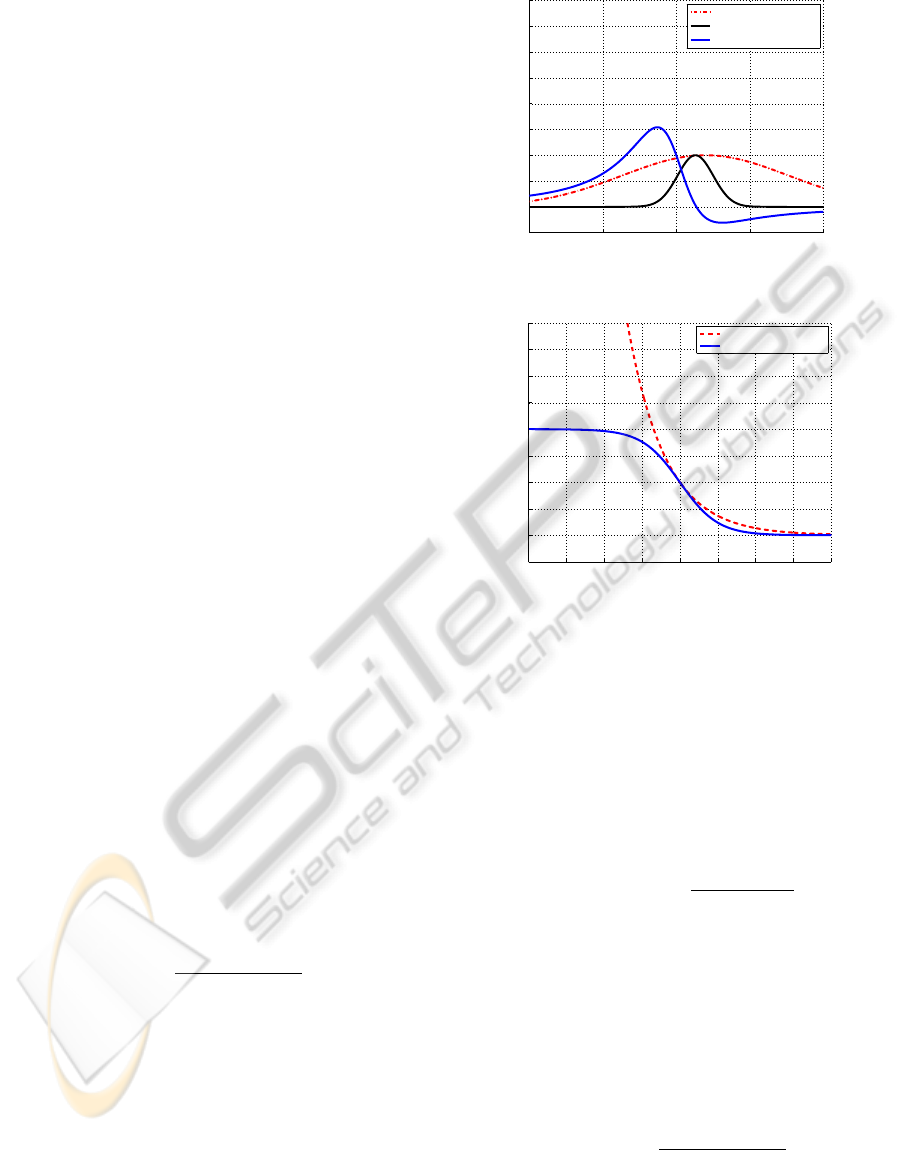
Figure 3(b) shows the different weight functions

and suggests that LogitBoost should be affected less

by examples far on the negative margin than the

exponential-loss algorithms.

3.2 Robust Boosting Algorithms

3.2.1 RobustBoost

RobustBoost is speciﬁcally designed to handle out-

liers (Freund and Science, 2009). RobustBoost, a

−4 −2 0 2 4

−0.5

0.5

1.5

2.5

3.5

Margin (yH)

Weight

RobustBoost (t=0.1)

RobustBoost (t=0.9)

TangentBoost

(a) Robust weight function

−4 −3 −2 −1 0 1 2 3 4

−0.5

0.5

1.5

2.5

3.5

Margin (yH)

Weight

AdaBoost/GentleBoost

LogitBoost

(b) Weight functions

Figure 3: Weight functions with respect to the margin.

This illustrates how much examples at different distances

from the margin are able to affect the decision boundary for

the different algorithms. In the GradientBoost formulation,

TangentBoost’s penalty for too correct examples results in

negative weights.

variation of BrownBoost, is based on the Boost-by-

Majority algorithm and has a very soft and non-

convex loss function

(x,y,t) = 1 − erf



v(x,y) − µ(t)

σ(t)



, (8)

where erf(·) is the error function, t ∈ [0,1] is a time

variable and µ(t) and σ(t) are functions

(t) = (σ

+ 1) exp (2(1 −t)) − 1 (9)

µ(t) = (θ − 2ρ)exp(1 − t) + 2ρ, (10)

with parameters θ, σ

and ρ. Equation 8 is differ-

entiated with respect to the margin to get the weight

function

(x,y,t) = exp



−

(v(x,y) − µ(t))

2σ(t)



. (11)

Figure 3(a) shows equation 11 for some values of t.

From these we can see the RobustBoost weight func-

tion changes over time. It is more aggressive in the

ImprovedBoostingPerformancebyExclusionofAmbiguousPositiveExamples

beginning and as t → 1, it focuses less and less on ex-

amples far away from the target margin θ. One inter-

pretation is that the algorithm focuses on all examples

early in the training stage, and as the algorithm pro-

gresses it starts ignoring examples that it has not been

able to push close to the target margin.

RobustBoost is self-terminating in that it ﬁnishes

when t ≥ 1. In our experiments we follow Freund’s

example and set σ

= 0.1 to avoid numerical instabil-

ity for t close to 1 and we obtain the parameters θ and

ρ by cross-validation.

3.2.2 TangentBoost

TangentBoost was designed to have a positive

bounded loss function for both positive and nega-

tive large margins, where the maximum loss for large

positive margins is smaller than for large negative

margins (Masnadi-Shirazi et al., 2010). To satisfy

these properties the method of probability elicitation

(Masnadi-shirazi and Vasconcelos, 2008) is followed

to deﬁne TangentBoost having a tangent link function

f (x) = tan (p(x) − 0.5), (12)

and a quadratic minimum conditional risk

∗

(x) = 4p(x)(1 − p(x)), (13)

where p(x) = arctan(H(x)) + 0.5. is the intermediate

probability estimate. Combining the above equations

results in the Tangent loss

(x,y) = (2arctan(v(x,y))− 1)

. (14)

We immediately see that the theoretical derivation

of TangentBoost and its implementation may have to

differ as the probability estimates p(x) ∈ [−π/2 +

0.5,π/2 + 0.5] are not proper, so that we only have

proper probabilities p(x) ∈ [0,1] for

H(x)

< 0.546.

This means that

H(x)

> 0.546 has to be handled

according to some heuristic, which is not presented

in the original paper (Masnadi-Shirazi et al., 2010).

In the original paper the Tangent loss is optimized

through Gauss steps, which similarly to LogitBoost

divides the importance of examples into two func-

tions. So as with the other algorithms we re-derive

(x,y) by using the GradientBoost method, and ob-

tain

(x,y) = −

4(2arctan(v(x,y)) − 1)

1 + (v(x,y))

. (15)

As seen in ﬁgure 3(a) this weight function gives

low weights for examples with large negative margin,

but it also penalizes large positive margins by assign-

ing negative weight to very conﬁdent examples. Since

(x,y) is actually the regression target this means

that the weak learner tries to ﬁt very correct exam-

ples to an incorrect label. It should be noted that

the Tangent loss is not optimized through the Gra-

dientBoost method in the original paper, but through

Gauss-Newton stepping and that the region of nega-

tive weights actually results in intermediate probabil-

ity estimates above 1.

4 A TWO-PASS EXCLUSION

EXTENSION

Our main point is that some fraction of the data, that

is easy to learn with a given feature and weak-learner

set, deﬁnes the core shape of the class - we call these

examples inliers. Then there are examples that are

ambiguous or uncommon so that they cannot be prop-

erly learned given the same representation, and trying

to do so might lead to overﬁtting, creating artefacts

or forcing a poorer deﬁnition of the shape of the core

of the class. We call these examples non-learnable or

outliers and illustrate their effect on training in ﬁgure

4. It is important to note that there might be hard ex-

amples with large negative margin during some parts

of training, but that eventually get learned without

overﬁtting. We refer to these examples as hard inliers,

and believe they are important for learning a well per-

forming classiﬁer.

Figure 4 illustrates that even if robust algorithms

are better at coping with outliers, they are still nega-

tively affected by them in two ways; The outliers still

have an effect on the decision boundary learnt, even

if their effect is reduced. Hard inliers are also subject

to the robust losses, thus having less inﬂuence over

the decision boundary than for non-robust losses, il-

lustrated in ﬁgure 2.

We propose that outliers and inliers should be

identiﬁed and handled separately so that the outliers

are only allowed to inﬂuence the training when al-

ready close to the decision boundary and therefore

can be considered as part of the core shape of the

class. This can be achieved with a very soft loss

function, such as the logistic loss or the Bayes con-

sistent Savage loss (Masnadi-shirazi and Vasconcelos,

2008). We use the logistic loss, since the Savage loss

gives more importance to slightly misclassiﬁed exam-

ples, rather than being symmetric around the margin.

Differentiating the logistic loss

(x,y) =

1 + exp (−ηv(x,y))

, (16)

with respect to the margin results in the weight func-

ICPRAM2013-InternationalConferenceonPatternRecognitionApplicationsandMethods

(a) AdaBoost

(b) TangentBoost

(d) AdaBoost with two-pass method

Figure 4: Example with ﬁve outliers. The decision bound-

aries the different algorithms produce in the presence of a

few outliers. The colour coding represents estimated prob-

ability p(y = 1|x). We can see how AdaBoost overﬁts to

the outliers, TangentBoost overﬁts slightly less and Robust-

Boost is able to handle the problem, even if it is less certain

around the boundary. Applying the two-pass method to this

problem results in a decision boundary that completely ig-

nores the outliers. (Best viewed in colour.)

tion

excl

(x,y) = ησ(−ηv(x,y))σ(η v(x, y)) (17)

where σ(·) is the sigmoid function. This weight func-

tion can be made arbitrarily thin by increasing the η

parameter. We call this function the exclusion func-

tion, as its purpose is to exclude outliers from train-

ing.

Since the inlier examples are considered learnable

we want the difﬁcult examples in the inlier set to have

high weight, according to the original idea of boost-

ing. For this reason all inliers should be subjected to

a more aggressive loss such as the exponential loss or

the binomial log-likelihood loss.

The main challenge is to identify the outliers in a

dataset. To do this we follow our deﬁnition of outliers

as non-learnable and say that they are the examples

with the lowest conﬁdence after completed training.

We therefore deﬁne the steady-state difﬁculty d(x

)

of the examples as their negative margin −v(x

)

after a fully completed training round, and normalize

to get non-zero values.

d(x

) =

(

max(H(x)) − H(x

) if y

= 1

H(x

) − min(H(x)) if y

= −1,

(18)

where H(x

) is the classiﬁcation score of example j.

This is referred to as the ﬁrst pass.

We order the positive examples according to their

difﬁculty d(x

) and re-train the classiﬁer, assigning a

fraction δ of the most difﬁcult examples to the out-

lier set and subjecting them to the logistic loss func-

tion. This second iteration of training is what we call

the second pass. Figure 1 shows some inlier and out-

lier examples for the bottle and chair classes. As we

have mentioned, what will be considered an outlier

depends on the features used. We use HOG in our ex-

periments (Dalal and Triggs, 2005), so it is expected

that the tilted bottles and the occluded ones are con-

sidered outliers, since HOG cannot capture such vari-

ation well.

As previously mentioned, our model for outlier

exclusion has two parameters: δ and η, where δ con-

trols how many examples will be considered as out-

liers and η controls how aggressively the outlier ex-

amples will be down-weighted. In our experiments

we choose a large value for η - effectively ignoring

outliers completely in the second round. The actual

fraction of outliers is both class and feature depen-

dent, so δ needs to be properly tuned. We tune δ

by cross-validation, yet we have noticed that sim-

ple heuristics seem to work quite well too. Figure

5 shows how the performance is affected by δ for

three different classes. We can clearly see that differ-

ent classes have different optimal values for δ, which

is related to the number of outliers in their datasets,

given the used features and learners.

5 EXPERIMENTS

We perform experiments on a large number of classes

to reduce the inﬂuence of random performance ﬂuc-

tuations. For this reason, and due to the availabil-

ity of a test set we select the VOC2007 dataset for

ImprovedBoostingPerformancebyExclusionofAmbiguousPositiveExamples

0 0.1 0.2 0.3 0.4 0.5

0.73

0.74

0.75

0.76

0.77

0.78

0.79

0.8

0.81

0.82

0.83

Exclusion fraction (δ)

Average precision

Motorbike class

Aeroplane class

Bottle class

Figure 5: Performance for different exclusion fractions

δ. Average precision on the test set, using the two-pass ex-

tension with LogitBoost for different exclusion fractions δ

and different classes. This ﬁgure illustrates that different

classes have different optimal exclusion fractions δ.

our experiments. Positive examples have bounding-

box annotations, so we crop and resize all positive

examples to have the same patch size. Since our

main focus is to investigate how our two-pass exclu-

sion method improves learning, we want to minimize

variance or tweaking in the areas not related to learn-

ing, and therefore choose a static non-deformable fea-

ture. We use the HOG descriptor (Dalal and Triggs,

2005) to describe the patches, since it has shown good

performance in the past, is popular within the vision

community, and its best parameter settings have been

well established.

To get the bounding boxes for the negative ex-

amples, we generate random positions, widths and

heights. We make sure that box sizes and aspect ra-

tios are restricted to values that are reasonable for the

positive class. Image patches are then cropped from

the negative training set according to the generated

bounding boxes. The patches are also resized to have

the same size as the positive patches, after which the

HOG features are computed. We then apply our two-

pass training procedure described in section 4 to train

a boosted stump classiﬁer.

We train boosted stumps using four different

boosting algorithms: AdaBoost, LogitBoost, Robust-

Boost and TangentBoost. AdaBoost and LogitBoost

are chosen for their popularity and proliferation in the

ﬁeld, and RobustBoost and TangentBoost are chosen

as they explicitly handle outliers. We also train an

SVM classiﬁer to use as reference.

For LogitBoost, AdaBoost and TangentBoost

there are no parameters to be set. For RobustBoost

two parameters have to be tuned: the error goal ρ

and the target margin θ. We tune them by holdout

cross-validation on the training set. With Tangent-

Boost we encountered an implementation issue, due

to the possibility of negative weights and improper

probability estimates. After input from the author of

(Masnadi-Shirazi et al., 2010) we manually truncate

the probability estimates to make them proper. Unfor-

tunately this forces example weights to zero for mar-

gins

v(x,y)

> 0.546, which gives poor results as this

quickly discards a large portion of the training set. To

cope with this and to obtain reasonable performance

we lower the learn rate of the algorithm. The linear

SVM is trained with liblinear (Fan et al., 2008), with

normalized features and using 5-fold cross-validation

to tune the regularization term C.

Jittering the positive examples is a popular way

of bootstrapping the positive dataset, but we believe

that this can also generate examples that are not rep-

resentative of that class. For this reason our two-

pass approach should respond well to jittered datasets.

We therefore redo the same experiments for the best

performing classiﬁer, augmenting the positive sets by

randomly generating 2 positive examples per labelled

positive example, with small random offsets in posi-

tions of the bounding box. We also mine for hard

negatives to get a complete picture of how the out-

lier exclusion extension interacts with bootstrapping

methods.

6 RESULTS

A summary of our results is that all boosting al-

gorithms except TangentBoost show consistent im-

provements for the experiments using our two-pass

extension, which can be seen in table 1. Before em-

ploying our two-pass extension LogitBoost performs

best with 11 wins over the other algorithms. After

the two-pass outlier exclusion LogitBoost dominates

even more with 15 wins over other outlier-excluded

algorithms and 13 wins over all other algorithms, in-

cluding LogitBoost without outlier exclusion.

6.1 Comparison of Boosting Algorithms

Table 1 also includes a comparison of the perfor-

mance between algorithms, showing performance

differences with and without the outlier exclusion.

Among the convex-loss algorithms LogitBoost per-

forms better than AdaBoost. The difference in per-

formance shrinks when our two-pass method is ap-

plied, which suggests that naturally occurring outliers

in real-world vision data affects the performance of

boosting algorithms and that those better able to cope

with such outliers have a greater potential for good

performance.

Even so, the robust algorithms perform worse than

LogitBoost. One reason for this could be that the ro-

ICPRAM2013-InternationalConferenceonPatternRecognitionApplicationsandMethods

Table 1: Performance of our experiments. Average Precisions of different classiﬁers, when applied to the VOC2007 test

set. The red box on each row indicates the best performing classiﬁer for the object class. Boldface numbers indicate best

within-algorithm-performance for excluding outliers or not. Red cells indicate total best performance for a given class. Wins

within algorithm (WWA) summarizes how often a learning method is improved by our extension, and Wins between algorithms

(WBA) summarizes how often an algorithm outperforms the others when having the same strategy for handling outliers. Note

that these results cannot be directly compared to results from the original VOC2007 challenge since we are performing image

patch classiﬁcation, using the annotated bounding boxes to obtain positive object positions.

mean Average Precision for each Algorithm

Adaboost LogitBoost RobustBoost TangentBoost Linear SVM

Class Use all Exclude Diff Use all Exclude Diff Use all Exclude Diff Use all Exclude Diff Use all Exclude Diff

plane 74.27 73.87 −0.40 73.13 74.09 0.97 72.49 72.23 −0.27 73.86 72.88 −0.98 74.04 72.01 −2.03

bike 87.59 88.24 0.66 87.85 88.43 0.58 86.86 87.98 1.12 86.81 86.80 −0.01 85.12 84.47 −0.66

bird 46.69 48.14 1.45 48.08 49.87 1.79 46.66 48.69 2.03 46.97 49.45 2.48 46.67 46.32 −0.34

boat 57.33 58.96 1.63 59.01 60.81 1.80 57.92 58.31 0.39 58.61 58.02 −0.59 57.00 56.94 −0.06

bottle 74.57 78.56 3.99 76.02 80.00 3.98 72.74 78.94 6.20 76.79 78.32 1.53 76.22 76.97 0.75

bus 86.79 86.18 −0.62 86.54 86.96 0.42 83.86 86.82 2.96 85.97 86.26 0.29 82.07 81.85 −0.22

car 87.05 87.73 0.68 88.32 88.32 0.00 88.26 88.14 −0.11 88.34 88.30 −0.04 86.22 85.93 −0.29

cat 49.45 49.18 −0.27 50.15 52.44 2.29 48.30 52.21 3.91 45.93 50.90 4.97 45.45 45.48 0.02

chair 67.68 69.36 1.68 68.26 69.93 1.66 66.06 68.91 2.85 67.42 68.09 0.67 64.08 63.94 −0.14

cow 81.90 83.25 1.35 81.99 83.85 1.87 81.83 82.71 0.87 81.50 80.63 −0.87 82.01 82.44 0.43

table 40.89 44.50 3.61 43.68 47.91 4.24 39.89 46.26 6.37 47.52 36.34 −11.18 28.35 28.09 −0.26

dog 47.83 51.56 3.73 51.27 51.68 0.41 47.66 52.24 4.58 51.25 50.21 −1.04 46.16 46.94 0.78

horse 76.09 76.10 0.01 78.83 78.84 0.01 77.72 78.28 0.56 75.20 76.20 1.00 75.55 75.77 0.21

motorbike 74.15 77.15 3.00 77.39 78.33 0.94 76.75 79.20 2.45 75.16 75.46 0.30 73.31 72.56 −0.76

person 58.56 63.64 5.08 65.16 67.03 1.87 60.17 65.09 4.92 66.04 67.02 0.98 60.86 61.84 0.98

plant 58.08 57.60 −0.48 60.46 60.51 0.04 56.87 59.62 2.75 59.28 58.23 −1.05 58.42 58.90 0.48

sheep 80.60 84.41 3.81 81.59 83.11 1.53 80.78 80.11 −0.66 84.38 82.01 −2.37 80.07 80.17 0.10

sofa 61.83 66.28 4.44 62.35 66.66 4.31 63.92 67.81 3.89 56.73 63.06 6.33 62.33 62.18 −0.15

train 73.18 76.91 3.74 73.98 76.74 2.75 73.13 77.26 4.13 73.87 74.74 0.87 71.82 72.10 0.28

tv 92.11 92.11 0.00 92.57 92.57 0.00 91.97 91.97 0.00 91.69 91.69 0.00 91.28 91.28 0.00

mean 68.83 70.69 1.85 70.33 71.90 1.57 68.69 71.14 2.45 69.67 69.73 0.06 67.35 67.31 −0.04

WWA 4 15 - 0 18 - 3 16 - 9 10 - 10 9 -

WBA 2 1 - 11 15 - 1 4 - 5 0 - 1 0 -

Table 2: Outlier exclusion with other dataset augmentation techniques. Positive jittering (J) and hard negative mining

(HN) improves performance even more in combination with outlier exclusion (OE).

mean Average Precision for each Object Class

Method plane bike bird boat bottle bus car cat chair cow table dog horse motor-

bike

person plant sheep sofa train tv mean

Default 73.13 87.85 48.08 59.01 76.02 86.54 88.32 50.15 68.26 81.99 43.68 51.27 78.83 77.39 65.16 60.46 81.59 62.35 73.98 92.57 70.33

J 75.64 87.33 49.34 57.59 76.68 88.69 88.29 49.95 68.28 83.63 48.25 51.87 79.78 77.83 66.17 63.59 82.86 64.51 78.08 92.55 71.55

J+OE 77.18 87.56 50.30 60.32 79.54 89.73 89.62 50.64 68.75 84.73 50.39 55.09 79.33 79.68 67.73 62.83 83.71 67.65 75.79 92.55 72.66

J+HN 76.31 87.35 50.85 61.10 80.08 89.41 89.62 51.23 68.93 84.88 49.35 53.08 80.90 79.67 65.78 61.98 81.39 64.07 76.18 92.98 72.26

J+HN+OE 77.73 87.46 48.60 59.76 80.67 89.37 90.07 53.76 70.11 86.55 51.24 53.99 80.92 77.78 67.54 62.39 85.60 66.83 77.38 92.98 73.04

bust algorithms make no distinction between outliers

and hard inliers, as previously discussed. Our two-

pass algorithm only treats ”non-learnable” examples

differently, not penalizing learnable examples for be-

ing difﬁcult in the early stages of learning.

Although RobustBoost has inherent robustness, it

is improved the most by our extension. One expla-

nation is its variable target error rate ρ, which af-

ter the exclusion of outliers obtains a lower value

through cross-validation. RobustBoost with a small

value ρ is more similar to a non-robust algorithm,

and should not suffer as much from the hard-inlier-

problem demonstrated in ﬁgure 2(c).

The SVM classiﬁer is provided as a reference

and sanity check, and we see that the boosting algo-

rithms give superior results even though only decision

stumps are used.

The higher performance of the boosted classiﬁer

is likely due to that combination of decision stumps

can produce more complex decision boundaries than

the hyperplane of a linear SVM. It is not surprising

that the linear SVM is not improved by the outlier

exclusion as it has a relatively soft hinge loss, tuned

soft margins, and lacks the iterative reweighting of ex-

amples and greedy strategy, that our argumentation is

based on.

ImprovedBoostingPerformancebyExclusionofAmbiguousPositiveExamples

6.2 Bootstrapping Methods in Relation

to Outlier Exclusion

We can see in table 2 that jittering has a positive effect

on classiﬁer performance and that our outlier exclu-

sion method improves that performance even more.

This shows that our two-pass outlier exclusion is com-

plementary to hard negative mining and positive jitter-

ing and could be considered as a viable data augmen-

tation technique when using boosting algorithms.

7 DISCUSSION AND FUTURE

WORK

We show that all boosting methods, except Tangent-

Boost, perform better when handling outliers sepa-

rately during training. As neither TangentBoost nor

RobustBoost reach the performance of LogitBoost

without outlier exclusion they might be too aggressive

in reducing the importance of hard inliers and not ag-

gressive enough for outliers. We must remember that

the problem addressed by the VOC2007 dataset does

not include label noise, but does deﬁnitely have hard

and ambiguous examples that might interfere with

learning the optimal decision boundary. Both Tan-

gentBoost and RobustBoost have previously shown

good results on artiﬁcially ﬂipped labels, but we be-

lieve that a more common problem in object classiﬁ-

cation is naturally occurring ambiguous examples and

have therefore not focused on artiﬁcial experiments

where labels are changed at random.

We notice that the improved performance from

excluding hard and ambiguous examples is corre-

lated with the severity of the loss function of the

method. AdaBoost, with its exponential loss func-

tion, shows large improvement down to TangentBoost

having almost no improvement at all. LogitBoost has

less average gain from the exclusion of outliers than

AdaBoost, but still achieves the best overall perfor-

mance when combined with the two-pass approach.

More surprising is that RobustBoost is improved the

most, in spite of its soft loss function. One explana-

tion is that there is an additional mechanism at work

in improving the performance of RobustBoost. Ro-

bustBoost is self-terminating, stopping when it has

reached its target error. When training on a dataset

with a smaller fraction non-learnable examples, it is

more likely to end up at a much lower target error,

which makes it more similar to other boosting algo-

rithms and lets it add more weak learners before ter-

minating.

We have seen that pruning of the hard-to-learn ex-

amples in a dataset without label noise can lead to

improved performance, contrary to the “more data is

better” philosophy. Our belief is that our method re-

moves bad data, but also that it reduces the impor-

tance of examples that make the learning more dif-

ﬁcult, in this way allowing the boosting algorithms

to ﬁnd better local minima. We still believe that more

data is better if properly handled, so this ﬁrst approach

of selective example exclusion should be extended in

the future, and might potentially combine well with

positive example mining, especially in cases where

the quality of the positives cannot be guaranteed.

8 CONCLUSIONS

We provide an analysis of several boosting algorithms

and their sensitivity to outlier data. Following this

analysis we propose a two-pass training extension that

can be applied to boosting algorithms to improve their

tolerance to naturally occurring outliers. We show ex-

perimentally that excluding the hardest positives from

training by subjecting them to an exclusive weight

function is beneﬁcial for classiﬁcation performance.

We also show that this effect is complementary to jit-

tering and hard negative mining, which are common

bootstrapping techniques.

The main strength of our approach is that clas-

siﬁcation performance is improved without any ex-

tra test-time cost, only at the expense of training-

time cost. We believe that handling the normal and

hard examples separately might allow bootstrapping

of training sets with less accurate training data.

We also present results on the VOC2007 dataset,

comparing the performance of different boosting al-

gorithms on real world vision data, concluding that

LogitBoost performs the best and that some of this

difference in performance can be due to its ability to

better cope with naturally occurring outlier examples.

ACKNOWLEDGEMENTS

This work has been funded by the Swedish Founda-

tion for Strategic Research (SSF); within the project

VINST

REFERENCES

Angelova, A., Abu-Mostafam, Y., and Perona, P. (2005).

Pruning training sets for learning of object categories.

In CVPR.

ICPRAM2013-InternationalConferenceonPatternRecognitionApplicationsandMethods

Bauer, E. and Kohavi, R. (1999). An empirical comparison

of voting classiﬁcation algorithms: Bagging, boost-

ing, and variants. MLJ.

Dalal, N. and Triggs, B. (2005). Histograms of oriented

gradients for human detection. In CVPR.

Dietterich, T. (2000). An experimental comparison of three

methods for constructing ensembles of decision trees:

Bagging, boosting, and randomization. MLJ.

Fan, R., Chang, K., Hsieh, C., Wang, X., and Lin, C. (2008).

LIBLINEAR: A library for large linear classiﬁcation.

JMLR.

Felzenszwalb, P., Girshick, R. B., McAllester, D., and Ra-

manan, D. (2010). Object detection with discrimina-

tively trained part-based models. PAMI.

Freund, Y. (1995). Boosting a weak learning algorithm by

majority. IANDC.

Freund, Y. (1999). An adaptive version of the boost by ma-

jority algorithm. In COLT.

Freund, Y. and Schapire, R. (1995). A decision-theoretic

generalization of on-line learning and an application

to boosting. In COLT.

Freund, Y. and Science, C. (2009). A more robust boosting

algorithm. arXiv:0905.2138.

Friedman, J. (2001). Greedy function approximation: a gra-

dient machine. AOS.

Friedman, J., Hastie, T., and Tibshirani, R. (2000). Additive

logistic regression: a statistical view of boosting. AOS.

Grove, A. and Schuurmans, D. (1998). Boosting in the

limit: Maximizing the margin of learned ensembles.

In AAAI.

Hays, J. and Efros, A. (2007). Scene completion using mil-

lions of photographs. TOG.

Kumar, M. P. and Packer, B. (2010). Self-paced learning for

latent variable models. In NIPS.

Kumar, M. P., Zisserman, A., and Torr, P. H. S. (2009). Ef-

ﬁcient discriminative learning of parts-based models.

In ICCV.

Laptev, I. (2009). Improving object detection with boosted

histograms. IVC.

Leistner, C., Saffari, A., Roth, P. M., and Bischof, H.

(2009). On robustness of on-line boosting - a com-

petitive study. In ICCV Workshops.

Long, P. M. and Servedio, R. A. (2008). Random classiﬁ-

cation noise defeats all convex potential boosters. In

ICML.

Masnadi-Shirazi, H., Mahadevan, V., and Vasconcelos, N.

(2010). On the design of robust classiﬁers for com-

puter vision. In CVPR.

Masnadi-shirazi, H. and Vasconcelos, N. (2008). On the

design of loss functions for classiﬁcation: theory, ro-

bustness to outliers, and savageboost. In NIPS.

Mason, L., Baxter, J., Bartlett, P., and Frean, M. (1999).

Boosting algorithms as gradient descent in function

space. In NIPS.

atsch, G., Onoda, T., and M

uller, K. (2001). Soft margins

for AdaBoost. MLJ.

Shotton, J., Fitzgibbon, A., Cook, M., Sharp, T., Finocchio,

M., Moore, R., Kipman, A., and Blake, A. (2011).

Real-time human pose recognition in parts from single

depth images. In CVPR.

Torralba, A., Fergus, R., and Freeman, W. T. (2008). 80

Million Tiny Images: a Large Data Set for Nonpara-

metric Object and Scene Recognition. PAMI.

Vezhnevets, A. and Barinova, O. (2007). Avoiding boosting

overﬁtting by removing confusing samples. In ECML.

Vijayanarasimhan, S. (2011). Large-scale live active learn-

ing: Training object detectors with crawled data and

crowds. In CVPR.

Viola, P. and Platt, J. (2006). Multiple instance boosting for

object detection. In NIPS.

Warmuth, M., Glocer, K., and R

atsch, G. (2008). Boosting

algorithms for maximizing the soft margin. In NIPS.

ImprovedBoostingPerformancebyExclusionofAmbiguousPositiveExamples