Constrained Predictive Control of MIMO System
Application to a Two Link Manipulator
Joanna Zietkiewicz
Institute of Control and Information Engineering, Poznan University of Technology, Poznań, Poland
Keywords: Predictive Control, Constraints, MIMO Systems, LQ Control.
Abstract: In the paper application of constrained predictive control to multi input, multi output system is presented.
The method is based on feedback linearization and LQ control. Constraints of the system are implemented
by interpolation of reference trajectory. Finding solution is a compromise between the unconstrained LQ
control and a constrained feasible control and is executed by minimization of one variable. The application
of the method to a two link manipulator is used to present advantages and limitations of the algorithm.
1 INTRODUCTION
Feedback linearization is a powerful technique that
allows to obtain linear model with exact dynamics
(Isidori, 1985), (Slotine and Li, 1991). Linear
quadratic control is well known optimal control
method and with its dynamic programming
properties can be also easily calculated (Anderson &
Moore, 1990). The combination of feedback
linearization and LQ control has been used in many
algorithms in Model Predictive Control applications
for many years and it is used also in present papers
(He De-Feng et al., 2011), (Margellos and Lygeros,
2010). Another problem apart from finding the
optimal solution on a given horizon (finite or
infinite) is the constrained control. A method which
use the advantages of feedback linearization, LQ
control and applying signals constraints was
proposed in (Poulsen et al., 2001). It rely in every
step on interpolation between the LQ optimal control
and a feasible solution – the solution that fulfils
given constraints. A feasible solution is obtain by
taking calculated from LQ method optimal gain for a
perturbed reference signal. The compromise
between the feasible and optimal solution is
calculating by minimization of one variable – the
number of degrees of freedom in prediction is
reduced to one variable.
2 THE TWO LINK
MANIPULATOR SYSTEM
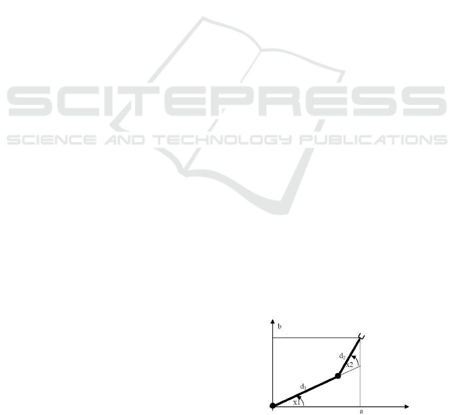
The considered system is the two link manipulator
(fig.1). It consists of two rigid links and two one
degree-of-freedom wrists, whose motion is in the
vertical axis. The objective of control is to move the
clutch of the manipulator from one position in two
dimensional space to the other. The output variables
are the two angles y
1
=x
1
and y
2
=x
2
. The coordinates
of the clutch can be obtained from kinematics
equations (1)
(1)
Figure 1: The two link manipulator system.
The dynamics of the system is represented by below
equations (2)
(2)
293
Zietkiewicz J..
Constrained Predictive Control of MIMO System - Application to a Two Link Manipulator.
DOI: 10.5220/0004122002930298
In Proceedings of the 9th International Conference on Informatics in Control, Automation and Robotics (ICINCO-2012), pages 293-298
ISBN: 978-989-8565-21-1
Copyright
c
2012 SCITEPRESS (Science and Technology Publications, Lda.)

where x
1
and x
2
are the angles, variables x
3
and x
4
are
the respective angular velocities, d
1
, d
2
are the
lengths of the links. The input variables u
1
and u
2
are
the moments of force in the wrists. Furthermore
(3)
represents Coriolis and centrifugal forces and
(4)
are the friction forces approximated by smooth
functions. The approximation is used to fulfil
conditions of feedback linearization method.
Masses and inertial forces are represented by M
matrix, where
(5)
The values of coefficients which appeared in
equations (3-5) are listed in tab.1.
Table 1: Coefficients of manipulator system.
link 1
link 2
I
i
[kg*m
2
]
1
1
m
i
[kg]
10
5
d
i
[m]
1
0.7
x
ci
[m]
0.5
0.35
y
ci
[m]
0
0
s
i
[Nm]
0.1
0.1
f
i
[kg*m
2
/s]
0.01
0.01
In considered system input variables u
1
and u
2
are
constrained by -1 and 1 Nm
(6)
2 CONTROL ALGORITHM
2.1 Feedback Linearization
Nonlinear equations of manipulator system are
smooth and the system has full relative degree. The
system has the same number of inputs and outputs.
Feedback linearization of the system can be
accomplished with diffeomorphism
(7)
and the new input variables
(8)
The inputs of the nonlinear system (2) are nonlinear
functions of v
1
, v
2
and the state x obtained from (8)
(9)
Consequently we obtain two identical linear systems
(10)
for which the theory of linear control can be applied.
2.2 Linear Quadratic Control
Each of the two linear systems is discretized with
sampling interval T
s
. In order to track the change of
set point the state is augmented by new variable with
included reference signal w
t
and each system is
described in form
tt
d
t
d
d
t
wv
1
0
0
1
0
1
B
z
C
A
z
tdt
y zC 0
(11)
The linear quadratic cost function can be written as
tk
kk
T
kt
RvJ ,
2
Qzz
(12)
and the solution
,
ttyt
wLv Lz
(13)
where L is the optimal gain obtained from Riccati
equation and
.0
T
dy
L CL
2.3 Constrained Predictive Control
The system equation (11) can be used as model
prediction equation to calculate the state for the
samples t+1=(k,…,k+H-1), on horizon H in the time
instant k. Constraints will be included into control
law by interpolation method in every predicted step.
It rely on using perturbed reference trajectory
(14)
In place of reference trajectory in equations (11 and
13). Then the prediction equation:
ktkktkt
d
kt
d
d
kt
pwv
|||||1
1
0
1
0
ˆ
0
ˆ
1
0
ˆ
B
z
C
A
z
(15)
And the control predicted values:
ICINCO 2012 - 9th International Conference on Informatics in Control, Automation and Robotics
294

,
ˆˆ
|||| ktktyktykt
pLwv zLL
(16)
Variable α
k
is calculated in instant k and is the same
for every predicted states and inputs on H, p
t|k
for
t=k,…,k+H-1 forms a vector p
H|k
. α
k
can adopt
values from 0 to 1 and p
H|k
is chosen in that manner
so the perturbed reference trajectory with α
t
=1
provides feasible, satisfying constraints solution for
the considered system. Whereas α
t
=0 corresponds
with unconstrained control. The aim is to minimize
variable α
t
on the horizon with respect to system
equations (15,16) and constraints (6). Since the two
systems (11) are considered, constrained values are
the functions of two variables α
k
I
and α
k
II
through
nonlinear equations (9) and (7) (linear in this
example, but nonlinear in general).
2.4 Feasible Trajectory
The perturbation vector p
H|k
providing feasible
solution can be obtain from previous k-1 step by
.1|1|
kHkkH
pp
(17)
With calculated α
t
for the n=3 dimensional system
(11) we can express the prediction equation from
(15) with used (16) in form:
),(
ˆˆ
|||1 ktkkttkt
pw
ΓzΦz
(18)
where
,
1
321
d
ddd
LLL
C
BBA
Φ
.
1
yd
LB
Γ
The initial perturbation p
H|i
for i at the beginning
of control application is calculated by using zero as
the reference signal and the initial state
corresponding to the step of original reference
signal. The method presented in (Poulsen et al.,
2001) of obtaining initial feasible perturbation
provided too large absolute values of control v at the
beginning of the predicted vector. The alternative
method is used in the paper with minimization of v
t
as a function of p
t
in (20).
For the state equation
ttt
pz ΓΦz
1
(19)
and initial z
0
=-(z
f
– z
k
),where z
f
– final stable state z
for w
k+1
, z
k
– initial state for control system,
additional cost function is used
tk
kpkp
T
kt
vRJ
2
zQz
(20)
where
tytt
pLv Lz
(21)
then the cost function has form
tk
kj
T
kkpkj
T
kt
pNzpRzQzJ 2
2
(22)
with
,RLLQQ
T
pj
,
yyj
RLLR
1
RLLN
T
j
(23)
The optimal gain K obtained by minimization (22) is
used to calculate initial perturbations p
t|i
, t=1,...H-1
.
|| itit
p Kz
(24)
Now we can describe the predicted variable z
k+l
and
predicted control law v
k+l
as a functions of initial and
final state, reference trajectory and one variable α
k
.
In equations k=i+1 is used:
)(
)(
)(
)(
ˆ
1
1
0
1
1
| kf
l
k
lk
k
k
k
l
klk
w
w
w
zz
ΓΦK
ΓΦK
ΓΦK
ΛΛzΦz
(25)
where
ΓΦΓΓΦΛ
1
l
)(
)(
)(
)(
0
0
ˆ
1
0
1
|
kf
l
d
k
lk
k
k
d
k
l
klk
w
w
w
v
zz
ΓΦK
ΓΦK
ΓΦK
C
ΛL
C
ΛLzLΦ
(26)
The linearized system of manipulator example (2)
consists of two linear equations (10) therefore in the
algorithm two prediction equations (25) and law
equations (26) are used. To avoid problems with
multivariable minimization it is assumed that α
k
is
equal to both subsystems, α
k
I
=α
k
II
.
3 PERFORMANCE OF THE
ALGORITHM
3.1 Simulations
Simulations was performed for the change of output
y
1
from 1.0489 to -0.0716 [rad] and y
2
from 0.9626
to 1.9284 [rad]. This is equivalent to the change of
Constrained Predictive Control of MIMO System - Application to a Two Link Manipulator
295
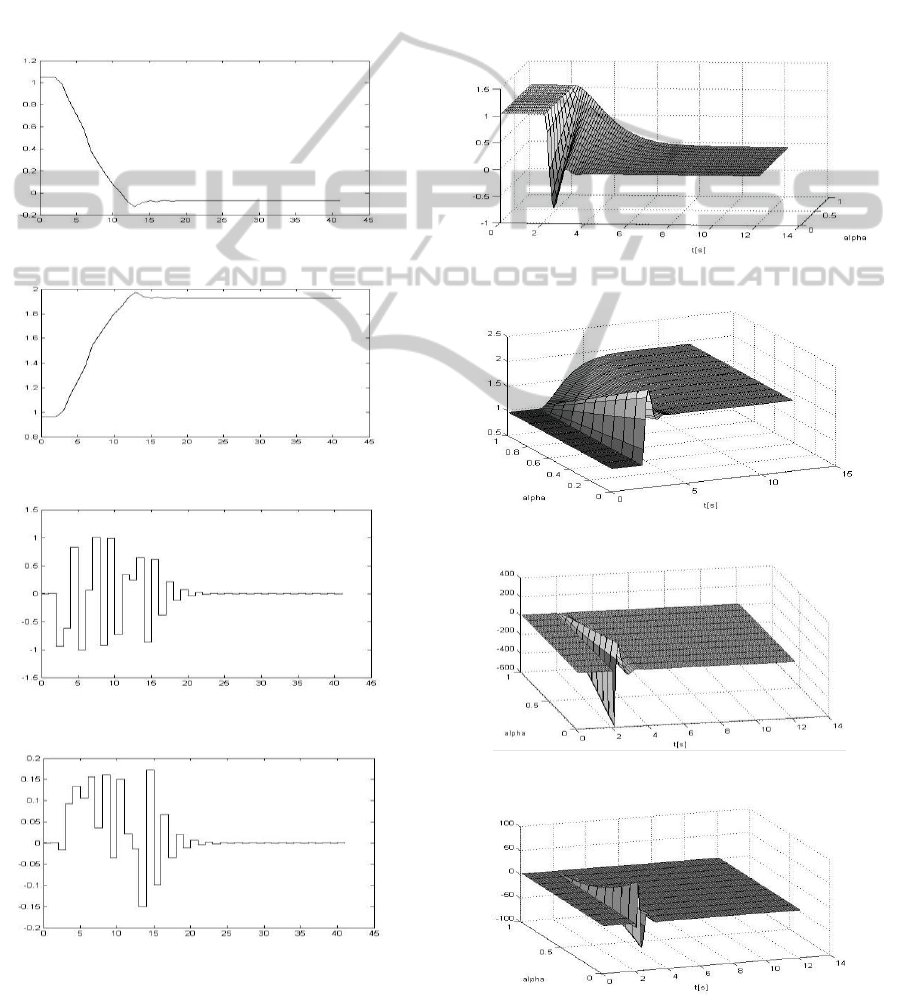
coordinates (a,b) from (0.2,1.5) to (0.8,0.6). The
weight matrices in cost function (12) for both
subsystems was chosen as Q=[0 0 0; 0 0 0; 0 0 1],
R=0.001 hence the emphasize in the minimization of
the difference between the set point and the output.
Remaining variables of the vector z are weighted
with 0, since constraints are coped while
minimization of α. R has to be positive define hence
the small value was chosen. The resulted trajectories
satisfied constraints, variables are changing fast and
without significant overshoot. Oscillations on inputs
charts are the effect of small R.
Figure 2: Output variable y
1
.
Figure 3: Output variable y
2
.
Figure 4: Input variable u
1
.
Figure 5: Input variable u
2
.
3.2 Variables as Functions of
In simulations only constraints of the two inputs
values was considered. In this section it can be seen
that for the remaining variables (the variables of
state x) can be considered constraints. The idea of
the algorithm is that by decreasing α the absolute
variables of inputs and consequently variables of
state are higher, the possibility of violating
constraints is greater. On figures (6-11) this
dependence of state variables and input on α is
presented.
Figure 6: Output variable y
1
in dependence on α.
Figure 7: Output variable y
2
in dependence on α.
Figure 8: Input variable u
1
in dependence on α.
Figure 9: Output variable u
2
in dependence on α.
ICINCO 2012 - 9th International Conference on Informatics in Control, Automation and Robotics
296
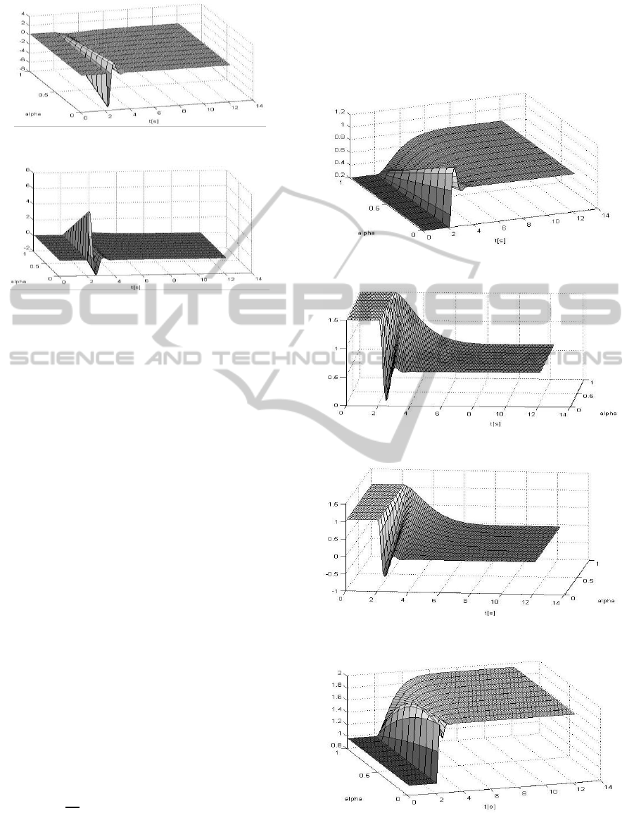
Figure 10: State variable x
3
in dependence on α.
Figure 11: State variable x
4
in dependence on α.
3.3 System with Coordinates as
Outputs
In order to present that the algorithm is not valid for
every feedback linearizable system of smooth
function the implementation of manipulator system
with different outputs was prepared. In this section
the outputs represents coordinates of the system that
is y
1
=a, y
2
=b. Then the system equations
(27)
The feedback linearization will be accomplished by
diffeomorphism
(28)
And new inputs
,
.
Two linear systems are obtained as in (10). The
system (21) has relative degree r=4, therefore there
are 4 variables the linear system and two additional
variables [z
5
z
6
]
T
=T
i
(x) has to be chosen. They have
to satisfy (Isidori, 1985), (Slotine & Li, 1991) equation
(29)
One of the possible choice is
(30)
The system (21) with performed linearization (22-
24) and used presented algorithm is not working
properly. The reason for this is that the dependence
of some variables on α is not monotonic as can be
seen on figures (12-17).
Figure 12: Output variable y
1
in dependence on α.
Figure 13: Output variable y
2
in dependence on α.
Figure 14: The variable x
1
in dependence on α.
Figure 15: The variable x
2
in dependence on α.
Constrained Predictive Control of MIMO System - Application to a Two Link Manipulator
297
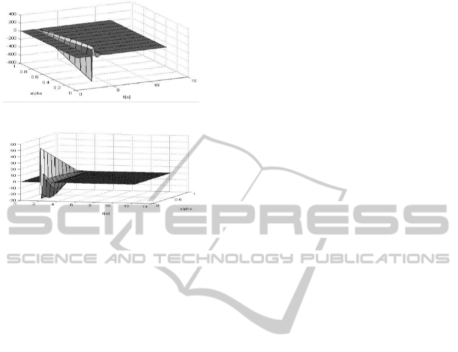
Figure 16: Input variable u
1
in dependence on α.
Figure 17: Input variable u
1
in dependence on α.
In this case variables x
2
and u
1
changes in the
undesirable manner as α increases. The main reasons
for this result is the chosen variable z
6
=x
1
+x
2
and
that nonlinear functions described inputs (9) are
fractions with nonlinear denominator dependent on
α.
REFERENCES
Slotine, J. E.; Li W. (1991). Applied Nonlinear Control,
Prentice-Hall, ISBN 0-13-040049-1, New Jersey,
USA
Poulsen, N. K.; Kouvaritakis, B.; Cannon, M. (2001).
Constrained predictive control and its application to a
coupled-tanks apparatus, International Journal of
Control, pp. 74:6, 552-564, ISSN 1366-5820
Isidori A. (1985). Lecture Notes in Control and
Information Sciences, Springer-Verlag, ISBN 3-540-
15595-3, ISBN 0-387-15595-3, Berlin, Germany
Margellos, K.; Lygeros, J. (2010), Proceedings of 49th
IEEE Conference on Decision and Control, ISBN
978-1-4244-7745-6, Atlanta, GA
He De-Feng, Song Xiu-Lan, Yang Ma-Ying, (2011),
Proceedings of 30th Chinese Control Conference,
ISBN: 978-1-4577-0677-6, pp. 3368 – 3371, Yantai,
China
Anderson, B. D. O.; Moore J. B. Optimal control. Linear
quadratic methods (1990), Prentice-Hall, ISBN 0-13-
638560-5, New Jersey, USA
ICINCO 2012 - 9th International Conference on Informatics in Control, Automation and Robotics
298
