Planning, Designing and Evaluating Multiple eGovernment

Interventions

∗

Fabrizio d’Amore

, Luigi Laura

, Luca Luciani

and Fabio Pagliarini

Dept. of Computer, Control and Mangement Engineering, Sapienza Univ. of Rome, Via Ariosto 25, 00185 Rome, Italy

INVITALIA Agenzia Nazionale per l’Attrazione degli Investimenti e lo Sviluppo d’Impresa S.p.A,

Via Boccanelli 30, Rome, Italy

Keywords:

eGovernment, Interventions Planning.

Abstract:

We consider the scenario where an organ of a public administration, which we refer as the decisionmaker,

is requested to plan one or more interventions in some framework related to the Information Society or the

eGovernment set of actions. We propose a methodology to support the decisionmaker in orienting, planning,

and evaluating multiple (partially overlapping) interventions. In particular, we address two main problems:

ﬁrst, how to decide the structure of the interventions and how to determine the relevant parameters involved;

second, how to set up a scoring system for comparing single interventions and its extension to the case of

multiple interventions. The methodology unexpectedly shows that it is not always the case that the best

outcome is the one obtained by the best projects. We formally model the problem and discuss its computational

complexity. Our approach is also effective in process of selecting, from a set of submitted proposals, the ones

to be funded.

1 INTRODUCTION

We consider a scenario aimed at planning and/or de-

signing interventions, namely the deﬁnition of the-

matic areas, categories of users and beneﬁciaries, ge-

ographic locations and speciﬁc goals constituting a

framework in which a decisionmaker wants to fund

new projects, during the process of setting up an ex-

plicit call. The decisionmaker is typically a speciﬁc

organ of the (central or local) public administration.

Such decisionmaker, in charge of assigning a give

amount of money, has to select the type of interven-

tion by mean of an articulated and complex decision

process, which includes kind of users to beneﬁt, type

of services and level of their interactivity, state/level

of existing and expected services, geographical and

socio-economical context, etc. It is clear that such a

decision process cannot be fully automated, but it can

get beneﬁts from the deﬁnition of guidelines and from

the availability of supporting tools that make faster

the so called “what-if” analysis.

Although the interventionswe consider pertain the

eGovernment, the Information Society and the ICT

areas, the results we present may apply to several oth-

∗

This work has been partially supported by the Italian

National Project POSI PON ATAS.

er areas.

In principle, the problem of making a decision can

be modeled as a problem of optimization, deﬁned by

an objective function to be minimized (or maximized)

under a set of constraints to be respected. The prob-

lem can be solved through mathematical techniques,

which can be rather complex, depending on the type

of objective function and constrains. In the case of

multi-objectivefunction the so-called Pareto optimum

(Fudenberg and Tirole, 2002) should be searched.

The number of variables and the complex constrains

to be modeled might turn the resulting optimization

problem intractable, that means no useful solution can

be found in real cases (Garey and Johnson, 1979).

Because of such issues we here propose a novel

approach, whose underlying model will be presented

in the next sections. We also address the problem

of evaluating interventions, by ﬁrst deﬁning the prob-

lem of evaluating a single intervention (Sect. 4), then

showing how to extend it to the case of multiple inter-

ventions (Sect. 5). We formally deﬁne this problem

and we prove that it belongs to the NPO complexity

class

, and therefore, if we want to efﬁciently solve it,

we must use some heuristics.

See the book of Papadimitriou (Papadimitriou, 1994)

for a classical reference on computational complexity.

d’Amore F., Laura L., Luciani L. and Pagliarini F..

Planning, Designing and Evaluating Multiple eGovernment Interventions.

DOI: 10.5220/0004071300850092

In Proceedings of the International Conference on Data Communication Networking, e-Business and Optical Communication Systems (ICE-B-2012),

pages 85-92

ISBN: 978-989-8565-23-5

 2012 SCITEPRESS (Science and Technology Publications, Lda.)

Table 1: Summary of the notation used in this paper.

notation meaning

B available budget for all the interventions

q number of interventions

budget for intervention i

number of projects to be funded in the intervention i

i, j

funding for project j of intervention i

i,1

i,p

ratio between min and max funding in intervention i

R B

ratio between the budgets of the interventions with min and

max budget

2 INTERVENTIONS AND

BUDGET

An intervention can be characterized by: the avail-

able budget, to be granted to co-funded projects; con-

straints on the employment of the budget, deriving

from laws and rules; types of objectives of fundable

projects; category of beneﬁciaries and their socio-

economical/territorial positions; type and impact of

the expected results.

The available budget is often an amount not sub-

jected to decision. This happens when an external

organization (e.g., the European Committee) makes

available to the decisionmaker an amount for co-

funding projects satisfying some speciﬁc require-

ments. The budget deﬁnes natural constraints on the

amounts to be assigned to the projects

and so it al-

lows to approximately dimension the interventions.

If resources are fairly distributes, it is easy to esti-

mate the number of projects to be funded, by deﬁning

the ratio between maximum and minimum funding.

Denoting the available budget by B, the number of

projects to be funded by p, the fund to be assigned to

the i-th project by B

and the ratio between the mini-

mum and the maximum funding by

r =

min

}

max

}

being 0 < r ≤ 1, it is possible to exploit mathematical

interpolation to dimension the amounts of the fund-

ings. In the case of linear interpolation we have

B =

∑

i=1

(max

} + min

})p

from which we get

max

} =

p(1+ r)

In the case of co-funding, the amount assigned to each

project is at least the 30–35% of the budget of the whole

project and therefore it determines its size.

If we re-number the projects accordingly to increasing

fundings we get

= B

− B

p− 1

( j − 1)

for j = 1, 2,..., p, with

2rB

p(1+ r)

Even if we have obtained these amounts by means

of a simple and arbitrary linear interpolation, they

are suitable to be the starting scheme of the decision-

maker. Subsequent reﬁnements will not cause, most

likely, substantial changes of the amounts.

In some cases, the decisionmaker can program in-

terventions by means of more than one call. Our ap-

proach still allows to determine the (base) amounts to

be assigned to the projects. We introduce in a more

compact form the used notation, assuming without

loss of generality that both interventions and projects

are numbered by increasing fundings. The linear in-

terpolation immediately gives

i,p

(1+ r

)

Such formula requires to know B

, which can be de-

termined by an analogous procedure.

q(1+ R)

, B

2RB

q(1+ R)

The searched value is

= B

− B

q− 1

(i− 1)

The decisionmaker can therefore ﬁx a few important

parameters, such as B, q, R and the r

’s, and use them

to compute the p

’s and B

i, j

’s. The whole process

could require some iterations, but allows to quickly

estimate the rough value of a few important quanti-

ties. This can be efﬁciently done exploiting a simple

spreadsheet.

ICE-B2012-InternationalConferenceone-Business

We conclude remarking the importance of recog-

nizing the relationships existing among different in-

terventions. In practice, if each intervention was in-

dependently planned, there would be no difference

between to plan q interventions and to plan q times

an intervention. What will make the quantum leap

is identifying the dependencies existing among dif-

ferent types of interventions, setting up a hierarchical

system that will allow to start well-coordinated and

highly correlated tasks, according to a bottom-up ap-

proach aiming at privileging the construction of basic

common infrastructures.

3 IMPACT ANALYSIS

We here introduce a methodology for carrying out

the analysis of the impact of a planned intervention.

It is based on the concept of indicator. Indicators

have been introduced in statistics and are currently

used in a variety of areas, among which the manage-

ment control (Smith, 2009); here we use indicators

for carrying out the analysis of the impact of interven-

tions. An indicator is a mathematical function deﬁned

over a ﬁnite or inﬁnite domain commonly deﬁned as

D = D

× D

× ··· × D

, where each D

is a ﬁnite set

of numbers (real, integer or natural) and n ∈ N de-

scribes the quantity of homogeneous data which we

want to get concise information from. In the man-

agement control, statistical indicators are used to get

concise information about some speciﬁc aspect of re-

ality; depending on the type of analysis we are carry-

ing on — pre-analysis, post-analysis, feasibility anal-

ysis, benchmarking etc. — many different categories

of indicators can be used. In the recent literature there

are several proposals providing sets of indicators, or-

ganized by category, level of aggregation, homogene-

ity, correlation etc. (see, e.g., (European Commission,

2010; eGEP, 2012; Ojo et al., 2005; Understand, 2006

)).

From what we discussed before, it is clear that the

Indicators Set (IS) plays a critical role in the whole

process of planning, designing, and evaluating inter-

ventions; the following points are therefore crucial:

1. The deﬁnition of a correct and complete Indica-

tors Set able to model the scenario.

2. The indicators in the IS must be easily measured

and constantly monitored before, during, and af-

ter the intervention. Information sources must be

reliable for the whole duration of the process.

3. In order to improve the reliability, the IS should be

chosen to be partially redundant, i.e. there should

be some correlation between different indicators

and, if possible, information sources should be

chosen to obtain independently values of corre-

lated indicators.

With distinct information sources providing the

values of the indicators, it is possible on one side to

havea precise picture of the real evolutionof the inter-

vention/project, on the other a variation in the correla-

tion between related indicators might point out some

errors in the measure or in the update of an indicator

and, in the long run, can help in the assessment of the

information sources themselves.

Given an indicators set I = {i

,..., i

}, we

deﬁne an aggregation (of the indicators) A =

,..., A

}, where A

⊆ I for any i and A

∩ A

0 for i 6= j; in other words, an aggregation is a par-

tition of I, conceptually based on a high level of ho-

mogeneity. From the decisionmaker point of view,

both indicators and aggregations belong to concep-

tual categories whose level is not sufﬁciently high.

The decisionmaker prefers to reason about concrete

objectives, directly related to beneﬁts for citizens, en-

terprises, concerns, public administration etc. When

deﬁning a main topic for an intervention (e.g., the area

of ICT) it is easy to deﬁne a set of (concrete) possi-

bly interesting objectives O = {o

,..., o

}. Once

O has been deﬁned, we expect it very slowly changes

as time passes, so that we can assume without loss of

generality O is ﬁxed. For each item o

∈ O it is possi-

ble to identify its correlations to some indicators in I

or, more simply, to elements in A.

In this way, when interested in an objective o

, the

decisionmaker can be easily informed about the in-

volved indicators, related to o

. It will be sufﬁcient

to make explicit all the correlations and store them

into some suitable supporting system. Notice that we

can consistently extend our assumption of static sets,

what leads us to static correlations. Identifying ele-

ments of sets and their correlations can be done once;

later, only limited maintenance will be required.

The decisionmaker is also interested in con-

textualizing information (according territory, socio-

economics, politics etc.). We assume for simplicity

one semantic coordinate of contextualization. Hence,

we introduce a set of contexts R = {r

,..., r

ℓ

}

(e.g., the main politic units, or regions, of a given

country). It is possible to introduce more sets of

contexts, all of them to be considered as orthogonal.

On the base of the context analysis, and of laws and

rules, high priority objectives can deﬁned, immedi-

ately identifying the involved indicators.

In order to describe all this knowledge we exploit

the mathematical concept of graph; for basic deﬁni-

tions on graphs (simple graph, tree, forest, walk etc.)

see for instance (Diestel, 2006). In particular we are

Planning,DesigningandEvaluatingMultipleeGovernmentInterventions

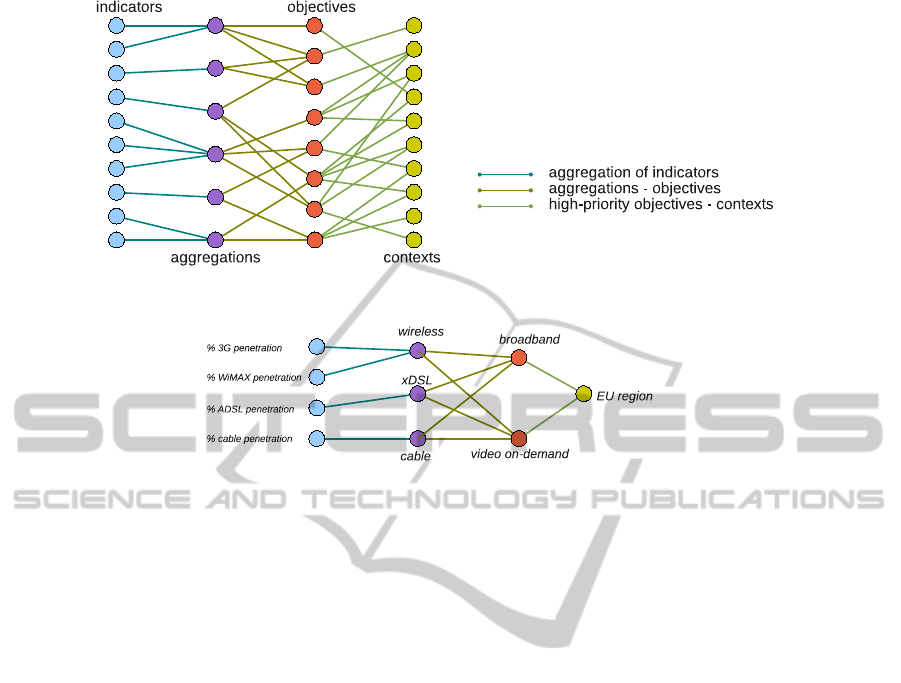
(a)

(b)

Figure 1: (a) A possible 4-parted graph, showing sets O, I, A and R. (b) Example of tree of monotonous walks.

interested in the notion of multipartite graph, deﬁned

as a simple graph G = (V, E) where

• V is partitioned into k subsets V

⊆ V, with

V and V

∩V

0 for i 6= j;

• there is no edge {u,v} if u and v belong to the

same subset of vertices.

In this case the graph is said to be k-parted.

We can use a 4-parted graph to represent sets I, A,

O and R, and to model the correlations existing among

their elements. We deﬁne a 4-parted graph whose set

of vertices is deﬁned as I ∪ A ∪ O ∪ R and it is par-

titioned into I, A, O and R, and whose edges are of

three types:

• Edges incident to vertices of A and I. They model

the structure of the aggregation of indicators.

• Edges incident to vertices of O and R. They

model the correlations between contexts and high-

priority objectives.

• Edges incident to vertices of A and O. They model

the correlations between high-priority objectives

and aggregations of indicators.

An example is given in Fig. 1 (a). Given such a graph,

by selecting any vertex all related information can be

automatically selected: it sufﬁces to ﬁnd the appropri-

ate set of walks.

Given a multipartire graph, we deﬁne a

monotonous walk as a walk having exactly one

vertex in every subsets of vertices. In the 4-parted

graph each monotonous walk is constituted by an

indicator, an aggregation of indicators, a context and

an objective. When the decisionmaker selects objec-

tive o

, the set of all monotonous walks containing

is immediately identiﬁed. It is easy to see that

such a set of walks deﬁne a tree, which we call “tree

of monotonous walks rooted at o

.” An example is

shown in Fig. 1 (b).

Our approach allows to capture the correlations

among the important concepts. Notice that the model

could be strengthened by quantifying the correlations,

so introducing a measure that can depend not only on

the two related concepts, but also on additional infor-

mation (contextualization, other strongly related indi-

cators etc.). A hypergraph (Berge, 1970), that gener-

alizes the concept of graph, seems to be a candidate

for such a quantitative model, however most of natu-

ral problems on hypergraphs are intractable. A sim-

pler way is to use weighted graphs, by introducing a

weighting function associating positive real numbers

(weights) to edges.

4 ASSIGNING SCORES TO

INTERVENTIONS

Our ﬁrst need is to deﬁne a Scoring System that, at a

ﬁrst glance, can be seen as a block box whose input

are: the target of the intervention (e.g. school, public

administration, concern etc.), the location of the in-

ICE-B2012-InternationalConferenceone-Business

tervention, the state of the indicators pre and post the

intervention, and the state of the average (national or

international) of the values of the indicators. The out-

put of the system is a score, representing the goodness

of the intervention/project.

We now brieﬂy describe some natural require-

ments that any Scoring System should satisfy; later

we propose a functional scheme that meets all the re-

quirements.

The input of the Scoring System, as described

above, can be formally detailed in the following way:

• The intervention target t ∈ T = { set of all the pos-

sible intervention targets }.

• The Indicator Domain D = D

× D

× · · · × D

where each D

is a subset of R, the set of real

numbers. Without loss of generality we can nor-

malize all the domains to the interval [0,1] ⊂ R.

• The state pre intervention is a vector i

,...i

), where i

∈ D

, i

∈ D

, .. . ,i

∈ D

• The state post intervention is a vector i

,...i

), where i

∈ D

, i

∈ D

, .. . ,i

∈ D

• The (national or international) average is a vec-

tor i

= (i

,...i

), where i

∈ D

, i

∈

, .. . ,i

∈ D

• The locality of the intervention is completely de-

scribed by the vector i

(state of the indicators be-

fore the intervention).

The output of the System is a score that, without

loss of generality, we can assume between 0 and 1;

therefore a Scoring System can be seen as a function

f : T × [0,1]

→ [0, 1]. Some natural requirements for

a scoring system are:

• If i

= i

, then f(t,i

) = 0 (zero score): if

a project does not improve any of the indicators

then its score is 0.

• If i

= (1,1. . . , 1), then f(t,I

) = 1 (max-

imum score): if an intervention/project raises all

the indicator the the maximum then its score is

maximum.

• Given two projects P1 and P2, with

= (i

,...i

+ ∆i

...i

) and i

,...i

...i

), then f(t,i

) ≥

f(t,i

) (non decreasing property): if

two different projects bring all the indicators to

the same values, except one, the project better

performing on that indicator should score better

(or equal

The score can be equal when, given a set of weights

representing the relative importance of the indicators, the

corresponding weight is 0.

4.1 A Proposed Scoring Function

In this section we present a scoring system that satis-

ﬁes the requirements described previously. In order to

do so, we ﬁrst need to deﬁne a way to model the inter-

vention target, and we decide to represent it as a vec-

tor of n weights t = (w

,..., w

), where w

∈ [0,1]

for j = 1,2,...,n. Here n is the number of indicators

and each weight w

represents the relative importance

of the indicator for the given target. The vector of

weights can be derived from the tree of monotonous

walks previously introduced, by identifying the ob-

jective (element of set O) which the target is aiming

at. In the case of more than objectives, the associated

forest of monotonous walks will be considered.

That being stated, the scoring system can be rep-

resented by the following function:

f(t,i

) =

t · (i

− i

)

t · (1

− i

)

(1)

where we have denoted by

the vector whose n

components are all equal to 1, by “·” the vector

product and by “−” the vector difference. We re-

call that, given two vectors v = (v

,..., v

) e w =

,..., w

) it holds that

v· w = v

· w

+ v

· w

+ ··· + v

· w

and

v− w = (v

− w

,..., v

− w

)

We prove now that this function satisﬁes all the re-

quirements:

• If i

= i

, then f(t,i

) = 0 (zero score):

f(t,i

) =

t · (i

− i

)

t · (1

− i

)

t · 0

t · (1

− i

)

= 0

where we have denoted by

the vector whose n

components are all equal to 0.

• If i

= (1,1...,1), then f(t,I

) = 1 (maxi-

mum score):

f(t,i

) =

t · (

− i

)

t · (1

− i

)

= 1

• Given two projects P1 and P2, with

= (i

,...i

+ ∆i

...i

) and i

,...i

...i

), then f(t, i

) ≥

f(t,i

) (non decreasing property):

f(t,i

) − f (t,i

) =

t · (i

− i

)

t · (1

− i

)

−

t · (i

− i

)

t · (1

− i

)

t · (i

− i

) −t · (i

− i

)

t · (1

− i

)

Planning,DesigningandEvaluatingMultipleeGovernmentInterventions

t · (i

− i

+ i

)

t · (1

− i

)

t · (i

− i

)

t · (1

− i

)

t · ((i

,. .., i

+ ∆i

,. .., i

) − (i

,. .., i

))

t · (1

− i

)

t · (0,0, ... , ∆i

,. .., 0)

t · (1

− i

)

≥ 0

We notice that this function does not keep into ac-

count the national (or international) average of the in-

dicators; the above deﬁnitions can be easily adapted

to include it.

5 EVALUATION OF MULTIPLE

AND OVERLAPPING

PROJECTS

So far we have considered the scoring of a single in-

tervention/project. We nowconsider the case in which

there are several distinct intervention/projects, poten-

tially overlapping. It is important to mention that,

when planning multiple projects, the value of the in-

dicators after the projects must be carefully analysed.

Let us provide an example: assume that, in a given

area, the broadband penetration is 30%; we have two

distinct projects, using distinct technologies, that have

been estimated to raise that value by, respectively,

35% and 45%. It is clear that, when estimating the

overall improvement of both projects, we cannot sim-

ply add the values, since this would lead to an un-

feasible value of 110%; neither we can estimate it to

100%, because it is reasonable that there should be

some overlapping in the population reached by both

projects, and therefore the real value might be some-

thing slightly bigger than 75%.

Therefore it is important to analyze the effect of

the multiple projects together,rather than simply sum-

ming up all the (estimated) effects. We now pro-

vide an example of a somewhat of a paradoxical ef-

fect: given a ranking of projects, it might happen that,

when we want to fund some of them, the best outcome

is when we choose the worst (in the ranking) projects.

Let us assume that we have 4 projects and 3 in-

dicators; for the sake of simplicity we assume that

(i) all the weights in the target vector are equal to 1

(t = (1,1, 1)), (ii) the initial value of all the indica-

tors is equal to 0 (i

= (0,0, 0)), (iii) the cost of each

project is unitary, and (iv) our budget is 2, i.e. we can

choose at most two projects amongst them. The post

intervention vectors for the projects are as follows:

• i

= (1.0,0.0, 0.0)

• i

= (0.9,0.0, 0.0)

• i

= (0.5,0.3, 0.0)

• i

= (0.5,0.0, 0.2)

It is easy to see that, if we compute the scoring func-

tion as deﬁned in 4, the outcome is

f(t,i

) > f(t,i

)

Since there is budget for two projects, it would

seem natural to fund P1 e P2; but let us now consider

the post intervention vectors for all the possible pairs:

• i

(P1+P2)

= (1.0,0.0, 0.0)

• i

(P1+P3)

= (1.0,0.3, 0.0)

• i

(P1+P4)

= (1.0,0.0, 0.2)

• i

(P2+P3)

= (1.0,0.3, 0.0)

• i

(P2+P4)

= (1.0,0.0, 0.2)

• i

(P3+P4)

= (1.0,0.3, 0.2)

It is clear that, if we have to choose only two

projects, the best outcome is when we fund P3 and

P4, that, considered alone are worst than P1 and P2,

but together are better.

We can formally deﬁne the problem above dis-

cussed (for the sake of simplicity we do not include

the intervention target t):

MULTIPLE PROJECTS EVALUATION (MPE).

Given in input:

• an initial scenario S, represented by the values of

a set of indicators I = (i

,...i

);

• a set of projects P = (p

, p

,... p

), each asso-

ciated with a cost (c

,...c

) and a post inter-

vention vector (v

,...v

); with I(p

) we de-

note the (estimated) values of the indicators after

the completion of project p

; if R ⊆ P with I(R)

we denote the (estimated) values of the indica-

tors after the completion of all the projects in R.

• a scoring function f : I → R;

• a real number b, representing the available bud-

get;

we look for a projects subset P

′

⊆ P, whose overall

cost is less than the budget, to maximize the scoring

function; more formally we look for a subset P

′

such

that:

•

∑

j:p

∈P

′ c

≤ b (budget constraint)

• ∀P

′′

⊆ P,P

′′

6= P

′

∑

j:p

∈P

′′ c

≤ b, f(P

′

) ≥ f(P

′′

)

(optimality constraint)

Can we design efﬁcient algorithms able to solve

this problem? Unfortunately, the problem belongs to

the NPO complexity class, as stated in the following

theorem:

ICE-B2012-InternationalConferenceone-Business

Theorem 1. The optimization problem MPE, as de-

ﬁned above, belongs to the NPO complexity class.

Proof. Let us now consider the decision problem as-

sociated with MPE, i.e. a the problem in which the

optimality constraint is replaced by the following

f(P

′

) ≥ S

where S is a parameter: now the problem is, given

also the parameter S, to ﬁnd a subset P

′

such that

f(P

′

) ≥ S. Let us denote by Decision-MPE (DMPE)

this decision problem. To prove that MPE ∈ NPO

we will show that its corresponding decision problem

DMPE is NP-complete (NPO is the complexity class

of the optimization problems whose decision versions

belong to NP (Ausiello et al., 1999)).

We recall that, in order to prove that a problem B

is NP-complete, it is sufﬁcient to show what follows

(see, e.g., (Garey and Johnson, 1979)):

1. There must be an NP-complete problem A such

that A ≤ B (A polynomially reduces to B).

2. B belongs to NP (e.g., by describing a polynomial

time algorithm for a non-deterministicTuring Ma-

chine able to solve it).

Let us now consider the following problem (Garey

and Johnson, 1979)

DOMINATING SET (DS).

INSTANCE: Graph G = (V,E) and a positive integer

K ≤ |V|.

QUESTION: Is there a subset V

′

⊆ V such that |V

′

| ≤

K, and such that every vertex v ∈ V −V

′

is joined to

at least one member of V

′

by an edge in E?

The Dominating Set problem is NP-complete

((Garey and Johnson, 1979)); let us nowdeﬁne a mod-

iﬁed version, where the underlying graph is directed:

DIRECTED DOMINATING SET (DDS).

INSTANCE: Directed graph G = (V,E) and a positive

integer K ≤ |V|.

QUESTION: Is there a subset V

′

⊆ V such that |V

′

| ≤

K, and such that every vertex v ∈ V −V

′

is joined to

at least one member ofV

′

by an outgoing edge in E?

We know prove that DMPE is NP-complete, and

our proof is articulated in the following steps:

1. DS ≤ DDS;

2. DDS ≤ DMPE;

3. DMPE ∈ NP.

Step 1: DS ≤ DDS. To show that DS reduces

to DDS we simply consider the following transfor-

mation: we change every undirected edge {a,b} of

the DS instance into the two directed edges (a,b) and

(b,a). It is easy to check that every solution of the

DDS instance obtained in this way is also a solution

of the related DS instance.

Step 2: DDS ≤ DMPE. To map the generic DDS

instance into one DMPE instance we will:

• each node v ∈ V is mapped into a project p ∈ P;

• each node v is also mapped into an indicator i ∈ I;

• the initial value of each indicator is equal to 0;

• for each node v ∈ V, for each outgoing edge (v, w)

we set equal to 1 the w-th components of the post

intervention vector associated with node v;

• for each node v ∈ V we also set equal to 1 the v-th

components of the post intervention vector asso-

ciated with the node;

• each project p

is associated with a cost c

=1;

• we set b = K;

• the objective function is f =

∑

∀i∈I,i≥1

1 (it counts

the number of indicators equal to 1);

• we set S = n = |V|.

Informally, the reduction is as follows: each node v

is mapped into a project able to cover all the nodes

reached by v, together with node v itself. The budget

is able to select only K nodes/projects and the param-

eter S is set in such a way that all the nodes must be

either dominators or dominated.

Step 3: DMPE ∈ NP. To show that DMPE ∈

NP is sufﬁcent to observe that this problem can be

solved by generating all the possible subsets of P and

by checking if one of them satisﬁes the constraint

f(P

′

) ≥ S. A non-deterministic Turing Machine can

simply guess at step i whether to include or not the

i-th project in the solution, and then check the con-

straint at the last step: therefore it takes linear time to

solve it, and this imply that DMPE ∈ NP.

6 CONCLUSIONS

We addressed the scenario where an organ of a public

administration, i.e. the decisionmaker, is requested

to plan one or more interventions in some framework

related to the InformationSociety or the eGovernment

set of actions.

We proposed a methodology to support the deci-

sionmaker in orienting, planning, and evaluating mul-

tiple (partially overlapping) interventions. In partic-

ular, we address two main problems: ﬁrst, how to

decide the structure of the interventions and how to

determine the relevant parameters involved; second,

how to set up a scoring system for comparing single

interventions and its extension to the case of multiple

interventions. The surprising result from this formal

Planning,DesigningandEvaluatingMultipleeGovernmentInterventions

analysis is that not always the best projects together

achieve the best outcome.

We formally modeled the problem and discussed

its computational complexity, showing that it is NP-

complete the problem of the selection of the projects

whose overall outcome is maximized.

REFERENCES

Ausiello, G., Protasi, M., Marchetti-Spaccamela, A., Gam-

bosi, G., Crescenzi, P., and Kann, V. (1999). Com-

plexity and Approximation: Combinatorial Optimiza-

tion Problems and Their Approximability Properties.

Springer-Verlag New York, Inc.

Berge, C. (1970). Graphes et Hypergraphes. Dunod, Paris.

Diestel, R. (2006). Graph Theory. Graduate Texts in Math-

ematics. Springer.

eGEP (2012). eGovernment Unit - DG Information Soci-

ety and Media - European Commission. eGovernment

Economics Projects - Measurements Framework. Fi-

nal Deliverable, available at http://rso.it/eGEP.

European Commission (2010). . Key ICT indicators for

the Member States, Norway and Iceland. i2010

Annual Information Society Report 2007, Vol. 3.

http://ec.europa.eu/information

society/eeurope/i2010.

Fudenberg, D. and Tirole, J. (2002). Game Theory. MIT

Press.

Garey, M. R. and Johnson, D. S. (1979). Computers

and Intractability: A Guide to the Theory of NP-

Completeness. W. H. Freeman and Company.

Ojo, A. K., Janowski, T., and Estevez, E. (2005). Deter-

mining progress towards e-government: What are the

core indicators? In Proc. of the 5th European Confer-

ence on e-Government, pages 312–322. ACL, Read-

ing, UK.

Papadimitriou, C. M. (1994). Computational complexity.

Addison-Wesley.

Smith, C. (2009). Economic indicators. In Wankel, C., edi-

tor, Encyclopedia of Business in Today’s World. SAGE

Publications, Inc., California, USA.

Understand (2006). Understand (European regions UN-

DER way towards STANDard indicators for bench-

marking information society). Methodological Hand-

book. Available at http://www.understand-eu.net/.

ICE-B2012-InternationalConferenceone-Business