Diffusion Tracking Algorithm for Image Segmentation

Lassi Korhonen and Keijo Ruotsalainen

Department of Electrical Engineering, Mathematics Division, University of Oulu, P.O. Box 4500, 90014 Oulu, Finland

Keywords:

Spectral Clustering, Image Segmentation, Diffusion.

Abstract:

Different clustering algorithms are widely used for image segmentation. In recent years, spectral clustering

has risen among the most popular methods in the ﬁeld of clustering and has also been included in many image

segmentation algorithms. However, the classical spectral clustering algorithms have their own weaknesses,

which affect directly to the accuracy of the data partitioning. In this paper, a novel clustering method, that

overcomes some of these problems, is proposed. The method is based on tracking the time evolution of the

connections between data points inside each cluster separately. This enables the algorithm proposed to perform

well also in the case when the clusters have different inner geometries. In addition to that, this method suits

especially well for image segmentation using the color and texture information extracted from small regions

called patches around each pixel. The nature of the algorithm allows to join the segmentation results reliably

from different sources. The color image segmentation algorithm proposed in this paper takes advantage from

this property by segmenting the same image several times with different pixel alignments and joining the

results. The performance of our algorithm can be seen from the results provided at the end of this paper.

1 INTRODUCTION

Clustering is one of the most widely used techniques

for data mining in many diverse ﬁelds such as statis-

tics, computer science and biology. One of the most

used applications for clustering algorithms is image

segmentation which plays a very important role in

the area of computer vision. The best known and

still commonly used methods for clustering are k-

means and fuzzy c-means (FCM) which are also

used in some quite new image segmentation algo-

rithms (Chen et al., 2008), (Yang et al., 2009). In

recent years, the spectral clustering based image seg-

mentation algorithms have risen among the most pop-

ular clustering based segmentation methods. There is

a large variety of spectral based clustering algorithms

available some of which are described in (Luxburg,

2007) and (Filippone et al., 2008). Basically, it is

possible to use any of them as a part of image segmen-

tation algorithms, but quite a little attention has paid

to the shortcomings of these spectral clustering based

segmentation algorithms, even if some of the limi-

tations are quite easy to reveal as shown in (Nadler

and Galun, 2007). These limitations affect straight-

forward also to the performance and accuracy of the

image segmentation process.

In this paper, we introduce a novel clustering ba-

based image segmentation algorithm that is closely

related to but have some signiﬁcant advantages com-

pared to the classical spectral clustering based meth-

ods. The algorithm is based on tracking diffusion pro-

cesses individually inside each cluster, or we can say

inside each image segment, through consecutive mul-

tiresolution scales of the diffusion matrix. The nature

of the algorithm supports combining segmentation re-

sults from different sources reliably. This enables the

statistical point of view to the segmentation process

and allows precise results also when using quite large

regions, patches, around each pixel when collecting

the local color and texture information. The paper

is organized as follows. First, in Section 2, we fa-

miliarize ourselves with some existing clustering al-

gorithms, and we will take a closer look at a couple

of spectral clustering algorithms that are commonly

used as a part of image segmentation algorithms. In

Section 3, we then introduce a new algorithm for clus-

tering and a new image segmentation algorithm will

be represented in Section 4. In Section 5, the clus-

tering and image segmentation results are reviewed.

Finally, some conclusions and suggestions for future

work will be provided in Section 6.

Korhonen L. and Ruotsalainen K..

Diffusion Tracking Algorithm for Image Segmentation.

DOI: 10.5220/0004055200450055

In Proceedings of the International Conference on Signal Processing and Multimedia Applications and Wireless Information Networks and Systems

(SIGMAP-2012), pages 45-55

ISBN: 978-989-8565-25-9

 2012 SCITEPRESS (Science and Technology Publications, Lda.)

2 SOME CLUSTERING

ALGORITHMS

There is a large variety of clustering algorithms avail-

able nowadays, and it is not possible to introduce

them extensively. The most common algorithms, k-

means, introduced in 1967 (Macqueen, 1967), and

FCM, introduced in 1973 (Dunn, 1973), are both

over 35 years old, and a lot of work to enhance

them has done also in recent years (Chitta and Murty,

2010), (Liu et al., 2010b), (Yu et al., 2010) and (Vintr

et al., 2011). Of course, many algorithms that are not

based on these two have been introduced during these

years. One of the newest algorithms is the linear dis-

criminant analysis (LDA) based algorithm presented

in (Li et al., 2011). The other interesting one, espe-

cially from our point of view, is the localized diffusion

folders (LDF) based algorithm presented in (David

and Averbuch, 2011). The LDF based algorithm can

be counted in to the category of spectral clustering

algorithms, and the hierarchical construction of the

algorithm has some similarities compared to the algo-

rithm presented in this paper.

As mentioned earlier, the spectral clustering algo-

rithms are commonly used as a part of image segmen-

tation algorithms nowadays, and this is due to their

excellent performance when dealing with data sets

with complex or unknown shape. The clustering al-

gorithm presented in this paper can also be thought as

a spectral clustering algorithm, although the spectral

properties of the diffusion matrix do not have to be

directly examined. Because of this relationship, we

introduce next a couple of classical spectral cluster-

ing algorithms that are also used as a baseline when

testing the performance of our algorithm later in this

paper.

2.1 The NJW and the ZP Algorithm

The main tools in the spectral clustering algorithms

are the variants of graph Laplacian matrices or some

relatives to them. One popular choice is the diffusion

matrix which is also known as the normalized afﬁnity

matrix. This matrix is also the core of the classical

Ng-Jordan-Weiss (NJW) algorithm (Ng et al., 2001)

and the Zelnik-Manor-Perona(ZP) algorithm (Zelnik-

manor and Perona, 2004). Next we will take a closer

look at these algorithms. Further information about

spectral clustering may be found in (Luxburg, 2007).

We use the notation A(x, y) for the entry of a ma-

trix A in a row x and in a column y through this paper.

Let X = {x

}

i=1

, x

∈ R

, be a set of N data points.

The clustering process using the NJW algorithm is

done as follows assuming that the number of clusters

M is available:

1. Form the weight matrix K ∈ R

N×N

of the simi-

larity graph G(V, E) where the the vertex set V =

}

i=1

represents the data set X = {x

}

i=1

. Use

Gaussian weights: K(i, j) = e

−

−x

where σ

is a ﬁxed scaling parameter.

2. Construct the diffusion matrix (i.e. the normal-

ized afﬁnity matrix) T = D

−

where D is a

diagonal matrix so that D(i,i) =

∑

i=1

K(i, j).

3. Find the M largest eigenvalues and the corre-

sponding eigenvectors u

. . . u

of the matrix T.

Form the matrix U ∈ R

N×M

with column vectors

4. Re-normalize the rows of U to have unit length in

the k · k

-norm yielding matrix Y.

5. Treat each row of Y as a point in R

and cluster

via the k-means algorithm.

6. Assign the original point x

to cluster J if and only

if the corresponding row i of the matrix Y is as-

signed to cluster J.

The ZP algorithm has a same kind of structure and is

based on the same basic principles as the NJW algo-

rithm. However, there are a couple of major advan-

tages in the ZP algorithm:

• The ﬁxed scaling parameter is replaced with lo-

cal scaling parameter so that K(i, j) = e

−

−x

where σ

= kx

− x

k, and x

is the n:th neighbor

of x

. This modiﬁcation allows the algorithm to

work well also in situations where the data resides

in multiple scales.

• The k-means step (5) can be ignored.

• The number of clusters can be estimated during

the process, so there is no need to know it before-

hand.

Both of these algorithms are based on same basic

ideas and if the ﬁxed scaling parameter is replaced

with local one, their accuracies on clustering are quite

the same, and both suffers from same shortcomings.

In next sections, we will represent a new algorithm

that overcomes some of these shortcomings.

3 NEW ALGORITHM FOR

CLUSTERING

The diffusion matrix T tells us how the data points are

connected with each other in a small neighborhood.

SIGMAP2012-InternationalConferenceonSignalProcessingandMultimediaApplications

The powers T

, t > 1, describe then the behavior of

the diffusion at different time levels t, and how the

connections between data points evolve through the

time. This process we call as the diffusion process.

We can make a couple of general assumptions

concerning the behavior of the diffusion process and

clustering. First of all, the spectral clustering algo-

rithms, including the algorithm presented here, are

generally based on the assumption that the diffusion

moves on faster inside the clusters than between the

clusters. Second, if we assume that the diffusion

leakage between clusters is relatively small, the diffu-

sion inside the clusters can reach almost the stationary

state, i.e. the state when the diffusion process has sta-

bilized inside the cluster.

The classical spectral clustering algorithms (in-

cluding the ZP algorithm) are based on comput-

ing the eigenvectors of the diffusion matrix (normal-

ized afﬁnity matrix) and assigning the data points

with help of these eigenvectors. However, these

kinds of methods suffer from limitations as presented

in (Nadler and Galun, 2007) where it was shown that

if there exist large clusters with high density and small

clusters with low density the clustering process may

fail totally. This is because the ﬁrst assumption does

not hold. Even if the situation would not be that bad,

the accuracy of the clustering process suffers from

this shortcoming when handling clusters with differ-

ent inner geometries. This problem may be partially

overcome by tracking diffusion processes through the

consecutive scales (time steps) inside each cluster in-

dividually, as will be shown.

The clustering algorithm presented here can be

separated in following phases:

1. Compute the distances between data points and

construct the diffusion matrix T using local scal-

ing or some other suitable scaling method.

2. Construct the multiresolution based on T up to the

level needed for the efﬁcient computation of the

powers of T.

3. Track the diffusion processes inside clusters using

the points and levels provided by the multiresolu-

tion construction process.

4. Do the ﬁnal cluster assignments and repeat the

tracking process if needed.

It is remarkable that all these phases are possible

to implement by using just basic programming rou-

tines without computing, for example, eigenvalues or

eigenvectors and without using any speciﬁc libraries

or functions such as k-means. However, if there is a

lot of noise present, the k-means step can be included

in the phases 3 and 4.

The phases 2-4 will be explained in more detail

in following sections, whereas the phase 1 will not

need any further explanations or details, as it is im-

plemented directly in the same manner as explained

in Section 2.

3.1 Phase 2: The Multiresolution

Construction

The multiresolution construction is needed for the ef-

ﬁcient computation of high powers of the diffusion

matrix T so that the time evolution of the matrix can

be analyzed. The multiresolution construction used in

here was ﬁrst introduced in (Coifman and Maggioni,

2006) and allows a fast, efﬁcient and highly com-

pressed way to describe the dyadic powers T

, p > 0,

of the matrix within a precision needed. The parame-

ter p indicates the multiresolution level and this time

resolution seems to be adequate and suitable for our

purpose.

We made previously an assumption that the dif-

fusion process is much faster inside the clusters than

between them. This means that the decay of the spec-

trum of the diffusion matrix constructed from the data

inside the cluster is far faster than that of the ma-

trix constructed from all the data. This causes the

euclidean distance between the columns of T

that

belong to a same cluster to approach towards zero,

and in some point, the numerical range of T

has

decreased so that only one column is needed for rep-

resenting each cluster. We can trace the columns that

survived last during the multiresolution construction

and use these points as an input to the next phase as

starting points for the tracking process.

3.2 Phase 3: Tracking the Diffusion

Process

The second assumption gives us a good starting point

for choosing the right multiresolution level, or we can

say the right moment of time, to stop the diffusion

process. The speed of the diffusion process inside

each cluster depends on the decay of the spectrum of

the diffusion matrix concerning that part of the data

set. This means that time needed by the diffusion pro-

cess to settle down inside each cluster varies, and it

would be necessary to have a possibility to choose the

stop level of the diffusion process for every cluster in-

dividually as mentioned earlier. This can be done in a

following way:

Let N

be an approximate number of data points

belonging to a cluster k, {s

}

k=1

a set of indices of the

columns tracked, or one can say the starting points,

during the diffusion process and {c

(i,k)

}

i=1

a small

DiffusionTrackingAlgorithmforImageSegmentation

set, n

≪ N

, of column indices of the data points

at the neighborhood of s

(inside cluster k). The set

(i,k)

} may be get from the support of columns s

the matrix T.

The process is started at level p = 1 by calculating

the approximation

from the multiscale represen-

tation constructed in the previous phase, normalizing

the columns tracked and storing them to the matrix

(1)

(l, k) =

(l, s

)

∑

i=1

, c

(i,k)

)

(1)

where l = 1, 2, . . . , N and k = 1, . . . , M. Next the data

points are assigned to clusters at this levelby the func-

tion

(p=1)

(l) = argmax

k=1,2,...,M

(1)

(l, k) (2)

where l = 1, 2, . . . , N. The decision whether to con-

tinue or to stop the diffusion process inside each clus-

ter is made as follows: If

(p=1,k)

∑

i=1

, c

(i,k)

)

∑

l=1

(p=1)

(l)=k

∑

j=1

( j, s

)

, (3)

k = 1, . . . , M, is smaller than the chosen threshold q,

stop the process inside the cluster k, else continue. In

an ideal case, there will not be any leakage between

clusters and R

(p,k)

approaches to 1 when the diffu-

sion moves towards the stationary state. This is ob-

vious because the mean of the points included in the

small neighborhood c

(i,k)

tends towards the mean of

all the points inside the support 1

(1)

(l)=k

. However,

the values above 1 as a threshold for making the de-

cision would be too high if there is a signiﬁcant leak-

age present, and, therefore, it would be reasonable to

choose 0.8 ≤ q ≤ 1.

If all the processes were allowed to continue, we

can let the diffusion processes move forward and step

to the next level p = 2 by computing the approxima-

tion

, updating the neighborhoods and computing

the matrix C

(2)

using the tracked columns of

. The

cluster assignments and the decision making process

will also be made in the same manner as at the previ-

ous level but using

instead of

. The tracking pro-

cess continues in this way through consecutive levels

until the level where some of the diffusion processes

will not be allowed to continue will be reached.

When the case R

(p,k)

< q appears, the correspond-

ing column of C

(p)

is transferred to the next level by

storing it to C

(p+1)

to the same place and will not be

updated by the normalized columns of the diffusion

matrix at that or other following levels. The process

is continued through the levels until all the individual

processes have stopped, and the cluster assignments

may then be found in g

)

where p

indicates the

ﬁnal level.

3.3 Phase 4: The Final Cluster

Assignments

In some cases, the diffusion tracking process started

from the points provided by the multiresilution con-

struction gives results accurate enough for ﬁnal clus-

ter assignments. However, one can ask, “Why not

to run in a loop the tracking algorithm and beneﬁt

from the information provided the previous tracking

phase?” This is a justiﬁable question because if we

can choose the tracked columns so that the diffusion

processes inside the clusters settles down as fast as

possible, we could also decrease the amount of leak-

age between clusters.

Let X

be the data set of size N

assigned to the

cluster k and T

the diffusion matrix constructed from

this data set. The rate of the connectivity between

points x

and x

inside a cluster k at level p can be

measured with diffusion distance

,k)

(i, j) = T

(i, i) + T

( j, j) − 2T

(i, j) (4)

as proposed in (Coifman and Lafon, 2006). Let the

diffusion centroid of the cluster k be the point with the

minimum mean diffusion distance inside the cluster:

(ct)

= argmin

i=1,2,...,N

∑

j=1

,k)

(i, j) (5)

where p

is the level where the diffusion was stopped.

The diffusion distance measures the connectivity be-

tween points of the data set so it is small if there are

a lot of connections, and vice versa. The point s

is,

therefore, the one where from the diffusion process

can spread most effectively through the cluster k.

New cluster assignments may then be got after a

new tracking process started from the centroids s

. In

most of the cases, there is not signiﬁcant change in the

cluster assignments after a couple of iterations.

4 IMAGE SEGMENTATION

ALGORITHM

Image segmentation is one of the most used applica-

tion for clustering algorithms. The development of

these clustering algorithms leads also to better image

segmentation algorithms some of which, quite recent

ones, are presented in (Tziakos et al., 2009),(Tung

SIGMAP2012-InternationalConferenceonSignalProcessingandMultimediaApplications

et al., 2010) and (Liu et al., 2010a). The segmenta-

tion algorithm presented here can be applied to any

kind of color or grayscale images. The size of the

image can be anything up to several megapixels, al-

though the used accuracy have to be adapted to the

image size. The segmentation process is based on di-

viding the image naturally to different areas by the

properties of the texture on these areas. Therefore, the

image has to be divided into patches, which are then

described to feature vectors. The algorithm consists

of following sequential phases:

1. Choose the patch size and the way to collect dif-

ferent layers from the image and form a stack

from the layers with correct alignment.

2. Extract the non-overlapping patches from the

layer stack and form the feature vectors from the

patches.

3. Choose the number of segments to be revealed

and ﬁnd out the patches to be tracked using the

diffusion tracking algorithm if not provided with

some other way.

4. Apply the diffusion tracking clustering algorithm

to all the layers individually using the patches pro-

vided by the previous phase as starting points.

5. Segment all the layers using the results of the pre-

vious phase and align the layers to a stack in the

same way they were collected.

6. Compute the mode value of each pixel from the

stack and form the segmentation given by these

values.

7. Find out the areas, where the segmentation was

not clear enough and pass them to next phase if

more accurate segmentation is needed. If not, skip

the next phase.

8. Go back to phase 1.

9. Perform mode ﬁltering on the image plane to the

result image.

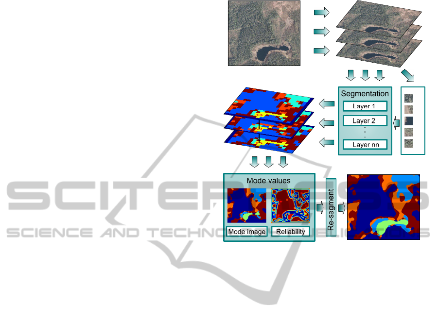
A simpliﬁed ﬂowchart representing the segmentation

process is shown in Figure 1. This algorithm is quite

simple to implement, and there are some interesting

parts in it. One of these, and maybe the most interest-

ing one, is the possibility to track the same patches in

different images or layers. In other words, the cluster

centroids are the same in all cases. This gives us the

possibility to join the segmentation results from dif-

ferent layers if we know the alignment of the layers.

The other interesting thing is that we can measure the

uncertainty of the segmentation process on the image

plane and run the segmentation procedure on these ar-

eas again with a ﬁner scale using a smaller patch size.

Next we will take a closer look at all the phases pre-

sented.

Patches tracked

Original image Extracted layers

Final result

Segmented layers

Figure 1: Image segmentation algorithm, ﬂow chart.

4.1 Phase 1: Collecting the Layers

We call the different pixel alignment choices as layers

in this context. Let us consider a case we have an

image of size N × M. The different layers from the

image can be collected by selecting all or a restricted

number of the sub images of size N − n× M− m from

the original image. For example, if we choose n =

1 and m = 1, it is possible to collect four different

sub images from the original one; the top, most left

pixel (1, 1) in the sub image can be chosen from a

pixel set (1, 1), (1, 2), (2, 1) and (2, 2) in the original

image. One crucial issue, which affects strongly on

the way to choose the layers, is the size of the patch

used for the texture description. The larger the patch

size, the more possible layers we have so that the non-

overlapping patches inside the layers are all different.

In case of the patch size 3 × 3 pixels, for example,

we have 9 possible different layers so that there are

not any similar patches inside the different layers. Of

course, it is not necessary, or even possible, to collect

all the layers when the patch size grows. One possible

way to choose layers from all possible choices in case

of patch size 3×3 and image size 12×12 is presented

in Figure 2. The layers are then stacked so that the

correct alignment remains.

DiffusionTrackingAlgorithmforImageSegmentation

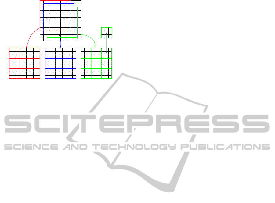
Layer 1 Layer 3Layer 2

12 x 12 image

Patch

Figure 2: Layer selection with patch size 3× 3 and original

image size 12× 12.

4.2 Phase 2: Forming the Feature

Vectors

All the non-overlapping square patches are then ex-

tracted from each layer separately and a description of

every patch is stored in a feature vector. The descrip-

tion is constructed in a following simple way. First

all pixels are sorted according to the value of each

pixel in a single color component and stored to a vec-

tor. This sorting process is done for every component

separately. Next all of these vectors are concatenated

so that the resulting vector is of size 3n

in case of a

RGB-image and a patch size n× n.

4.3 Phase 3: Choosing the Patches to be

Tracked

One very important thing on ensuring the proper

working of the diffusion tracking algorithm used for

clustering is the choice of the starting points for the

diffusion processes inside each cluster, or we can say

inside each image segment in this case. When seg-

menting an image, a natural way to choose these start-

ing points or patches is to manually select patches

from the areas to be treated as different segments.

This is possible because the tracking algorithm allows

the patches tracked to be ﬁxed. Of course, it is possi-

ble to search these patches automatically as explained

previously in Section 3. In that case, only the num-

ber of different segments and the set of layers, where

from to search the patches, have to be given to the

algorithm.

4.4 Phase 4: Clustering

The clustering phase is done for each layer separately

using the diffusion tracking algorithm. This is possi-

ble because the tracked patches can be added to each

of the sets of patches formed from different layers so

that all the tracking processes can be considered com-

parable. This property allows also the use of efﬁcient

parallel computing in the clustering phase because all

the different tracking processes can be ran indepen-

dently without any exchange of data between them.

This is quite an important issue because the clustering

phase is the most demanding one computationallyand

thus the most time-consuming one. After the cluster-

ing process, every single patch is connected and la-

beled to one of the clusters which represents different

types of image textures in this case.

4.5 Phase 5: Layer Segmentation

The labeled patches are then mapped back to an image

of same size as the original one so that we have a set

of different segmentation results, one per every layer,

from that image. These different segmented layers

are stacked so that the alignment of the layers corre-

sponds the original alignment.

4.6 Phase 6: Joining the Results

The segmented layer stack gives us a lot of possibili-

ties to choose the ﬁnal label of each pixel in the result

image. A straightforward and reasonable way to ap-

proach this problem is to use the statistical point of

view. There are a lot of propositions for the label of

each pixel, so why not to choose the one which has

the most of votes. This idea is very easy to implement

just by choosing the mode value from the set of labels

of each pixel. This solution has proven to be very re-

liable and stable also in experimental tests. Because

of the different alignment of the layers, there will be a

narrow border area around the image where the num-

ber of labels is smaller than elsewhere and, therefore,

the reliability suffers a bit on that area.

4.7 Phase 7: Measuring the Reliability

of the Segmentation

As presented earlier, a set of different labels is at-

tached to every single pixel. The reliability of the

segmentation result of each pixel is then revealed sim-

ply by examining the distribution of the labels, pixel

by pixel. If the number of votes for the mode value

at each pixel clearly outnumbers the other values, the

chosen label can be considered reliable and the seg-

mentation of that pixel ﬁnal. In other case, the pixel

examined is tagged as uncertain one and may need

further processing and re-segmentation. Choosing the

threshold between uncertain and certain labeling is

SIGMAP2012-InternationalConferenceonSignalProcessingandMultimediaApplications

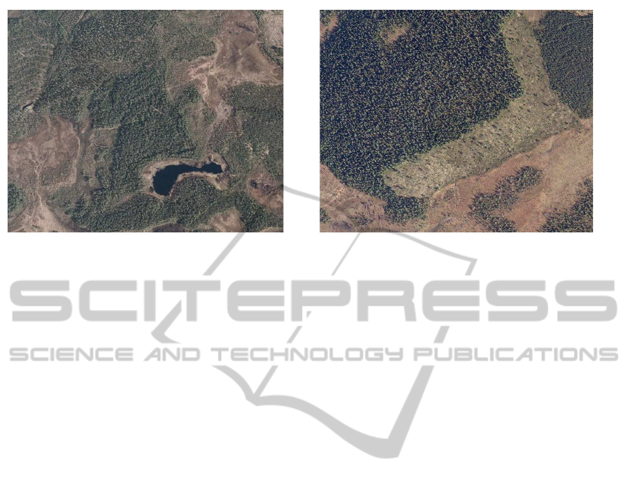
Figure 3: Original aerial images.

a tradeoff between more accurate results and more

computing time. The experimental tests have shown

that a good choice as a threshold could be as high as

75% of all votes for the won label.

4.8 Phase 8: Loop

If more accurate results were needed, the areas to be

re-segmented are then passed to the phase 1 where

the patch size is scaled downwards compared to the

previous round. The patches tracked are also scaled

down and kept as a starting points for the next round

clustering process.

4.9 Phase 9: Smoothing

After the accuracy wanted is achieved, the remaining

phase is to smooth the image. This may be necessary

due to the single separate pixels or small pixel groups

on the re-segmented areas. The ﬁltering method pro-

posed here is related to the median ﬁltering on the

image plane, but instead of using the median value of

the pixel neighborhood, the mode value is used.

5 EXPERIMENTAL RESULTS

The performance of the clustering algorithm pre-

sented in this paper was tested together with the ZP al-

gorithm based segmentation algorithm using an aerial

image as a data source. The ZP algorithm outper-

forms usually the classical NJW algorithm and there-

fore the results achieved with classical NJW are omit-

ted. However, when clustering some of the data sets

extracted from the image, the ZP algorithm provided

by authors of (Zelnik-manor and Perona, 2004) failed

totally. Therefore, the performance of our algorithm

is compared also with the NJW algorithm enhanced

with local scaling. Neither ZP nor NJW algorithm

supports directly the image segmentation procedure

presented here, so the ﬁnal segmentation results using

these clustering methods could not be provided this

time.

5.1 Aerial Image Segmentation

The image segmentation algorithm presented in this

paper is based on clustering patches collected from

an image. In this experiment, two color aerial images

are used as a source of data to be clustered and as an

example cases for the segmentation algorithm. Fig-

ure 3 represents the aerial images to be segmented.

The images are RGB images of size 750× 900 pixels

(height×width) and are acquired from the National

Land Survey of Finland (2010). Only a slight con-

trast enhancement has been done for both of the im-

ages before the segmentation process. The main goal

of the segmentation process is to reveal the areas of

different terrain types such as lakes, forests of differ-

ent densities and bogs using the information provided

by rectangular patches extracted from the image. The

number of different terrain types is chosen to be ﬁve

in both of the cases. This choice is reasonable when

looking at the images: There is a clearly visible wa-

ter area, woodless bog areas and the forest areas can

be divided quite clearly to three types with different

densities in the image on the left side, whereas there

are four different types of forest areas and a woodless

bog area in the image on the right side.

To provide some proof of the good performance

in the clustering accuracy of the proposed method,

our algorithm is compared with the ZP algorithm and

also with the NJW algorithm with local scaling be-

cause the ZP algorithm failed totally in some tests

DiffusionTrackingAlgorithmforImageSegmentation

2 4 6 8 10 12 14 16 18

−0.1

−0.05

0.05

0.1

0.15

−0.1

−0.05

0.05

0.1

0.15

−0.2

−0.1

0.1

0.2

−0.1

−0.05

0.05

0.1

0.15

−0.1

−0.05

0.05

0.1

0.15

−0.2

−0.1

0.1

0.2

−0.1

−0.05

0.05

0.1

0.15

−0.1

−0.05

0.05

0.1

0.15

−0.2

−0.1

0.1

0.2

2 4 6 8 10 12 14 16 18 20

−0.1

−0.05

0.05

0.1

−0.1

−0.05

0.05

0.1

0.15

−0.2

0.2

0.4

0.6

−0.1

−0.05

0.05

0.1

−0.1

−0.05

0.05

0.1

0.15

−0.2

0.2

0.4

0.6

−0.1

−0.05

0.05

0.1

−0.1

−0.05

0.05

0.1

0.15

−0.2

0.2

0.4

0.6

5 10 15 20 25

−0.1

−0.05

0.05

0.1

−0.1

−0.05

0.05

0.1

0.15

−0.2

0.2

0.4

0.6

−0.1

−0.05

0.05

0.1

−0.1

−0.05

0.05

0.1

0.15

−0.2

0.2

0.4

0.6

−0.1

−0.05

0.05

0.1

−0.1

−0.05

0.05

0.1

0.15

−0.2

0.2

0.4

0.6

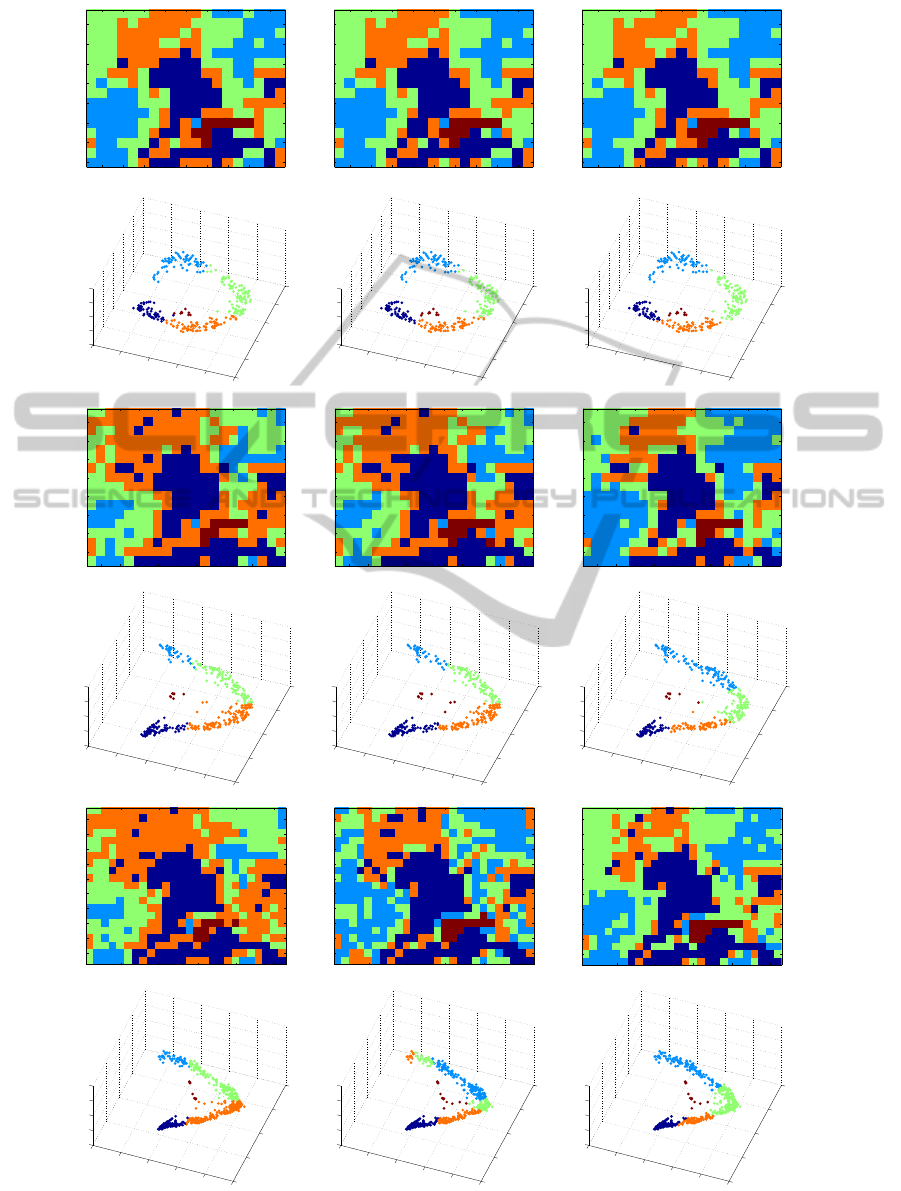
Figure 4: Rows 1,3,5: Segmentation results with patch sizes 44 × 44, 40 × 40 and 33 × 33. From left: NJW, ZP, and our

algorithm. Rows 2,4,6: The same results embedded via the ﬁrst three eigenvectors of the diffusion matrix.

SIGMAP2012-InternationalConferenceonSignalProcessingandMultimediaApplications

as can be noticed in following results. The compar-

ison was done by segmenting a single layer extracted

from the aerial image on the left side in Figure 3.

Figure 4 shows the results using three different patch

sizes. The patch sizes are chosen so that visible dif-

ferences can be noticed. In addition to the segmenta-

tion results, there are also the embeddings via the ﬁrst

three eigenvectors of the diffusion matrix presented,

and these embeddingsshow even more clearly the dif-

ferences between algorithms. The dark red color rep-

resents water areas, light blue woodless areas, green

sparse forest areas, orange forest areas with medium

density and dark blue dense forests.

All the algorithms perform quite well when us-

ing the patch size 44 × 44 and the reason for that is

clearly seen on embeddings via the eigenvectors. The

ﬁve different clusters are all well separated, and this

guarantees the good performance also for the spectral

clustering algorithms like NJW and ZP.

Changing the patch size a little bit smaller to size

40× 40 makes the clustering problem much more dif-

ﬁcult. Both the NJW and ZP algorithm fail to reveal

the edges of the green and orange areas and this can

also be seen on embeddingswhere the border between

these areas go through the densest part of the data

cloud. The performance of our algorithm suffers also

a little bit, but the result is still quite close to the one

achieved with larger patch size.

The most interesting results are found when us-

ing patch size 33 × 33. The ZP algorithm fails totally

while mixing the green and orange areas with each

other. The reason for that is unclear, and it is quite

surprising because the NJW algorithm works as sup-

posed. However, the NJW algorithm is not capable

of revealing the edges between the orange and green

areas. The clusters it founds for these areas look like

dipoles when looking at the embedding ﬁgure. Our

algorithm succeeds quite similarly as in other cases

presented and does the segmentation in a very natural

way when compared to the original image.

It is quite surprising to see from Figure 4 that our

algorithm can ﬁnd quite well the natural patches to be

tracked using just a single layer. This is a very ben-

eﬁcial property because the segmentation of a single

layer provides quite a good hunch about the ﬁnal re-

sult if the same patches are tracked through all the lay-

ers, as it can be seen later. However, there are some

possibilities to improve the way to ﬁnd the patches

tracked. One simple way is just to combine all the

patches from several layers together and try to search

the starting points from that set.

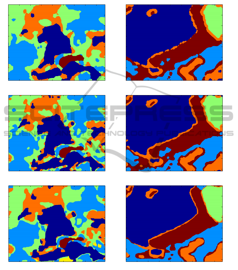
In the case of the left side image in Figure 3, the

ﬁnal segmentation result presented is achieved using

the patch size 40× 40 in the ﬁrst loop and 20× 20 in

the second, and the patches tracked are the same as

found and used in the single layer case in Figure 4. In

the case of the right side image, patch size 35×35 was

used in the ﬁrst loop and 21 × 21 during the second

one. The effect of the second loop is quite clear, and

the improvement in the accuracy compared with the

result after the ﬁrst loop is obvious, as can be seen

when comparing the results in Figure 5.

The ﬁnal results are quite impressive, and when

compared with the original images or the manually

segmented images showh in Figure 5, only a slight

errors may be noticed. The left side image was obvi-

ously more difﬁcult to segment, thus there is one ob-

vious error on surroundings of the small lake, where

there can be seen a clear open area around the lake

in the original image, but the segmentation algorithm

fails to reveal it. The second one can be found in the

bottom center part of the image where the wet bog is

segmented as a dense forest. However, it is quite difﬁ-

cult to decide the ground truth of the right class for the

wet bog areas. Therefore, these areas are marked with

yellow color in the manually segmented image. The

natural edges of the different terrain types are found

as they are in real and, for example, the borders of the

lake are nearly as accurate as they can be. The seg-

mentation results in the case of the right side image

contain some small mistakes in surroundings of the

dense forest nose, as can be noticed when compar-

ing the ﬁnal result with the manually segmented and

the original image. The orange border stripes around

the forest areas may also be thought as mistakes, but

that is not so obvious. The percentage of similarly

segmented pixels between the manual and automatic

segmentation in the more difﬁcult case was 80.1 %

and in the easier case, 89.5 %. The accurate manual

segmentation in these kind of cases is an impossible

task, so the importance of these values can be ques-

tioned.

6 DISCUSSION AND

CONCLUSIONS

The results of our algorithm are really promising, al-

though there are a lot of possibilities to develop it

still. One main target to develop is the construction of

the multiresolution which is not optimized for clus-

tering at all and may produce, in some cases, bad

starting points for the tracking algorithm. The use

of biorthogonal diffusion wavelets (Maggioni et al.,

2005) instead of orthonormal diffusion wavelets will

also be studied carefully; there are some stability is-

sues which preventedthe use of them in our algorithm

in this time. The use of more dense time resolution

DiffusionTrackingAlgorithmforImageSegmentation

100 200 300 400 500 600 700 800

100

200

300

400

500

600

700

100 200 300 400 500 600 700 800

100

200

300

400

500

600

700

100 200 300 400 500 600 700 800

100

200

300

400

500

600

700

100 200 300 400 500 600 700 800

100

200

300

400

500

600

700

100 200 300 400 500 600 700 800

100

200

300

400

500

600

700

100 200 300 400 500 600 700 800

100

200

300

400

500

600

700

Figure 5: First row: Segmentation results after the ﬁrst loop. Second row: The ﬁnal segmentation results. Third row:

Segmentation results with manual segmentation.

and the coherence measure presented in (Nadler and

Galun, 2007) as a part of our algorithm will also be

studied like the use of different similarity measures

also. The aim of using the coherence measure is to try

ﬁnd out the optimal number of clusters and, in other

hand, to prevent the appearing of unwanted clusters.

The algorithm for image segmentation presented

in this study has many interesting advantages and

properties compared to the traditional spectral or

other clustering based algorithms. The more com-

prehensive test results about the accuracy of the clus-

tering algorithm will be presented in upcoming ar-

ticles. However, a lot of improvements are possi-

ble to make to the existing algorithm some of which

SIGMAP2012-InternationalConferenceonSignalProcessingandMultimediaApplications

are already under implementation phase. The crucial

points, which are quite easily improved, are the search

of the patches to be tracked and the actual cluster-

ing algorithm, as mentioned earlier. Even if there are

some easily improved things in our algorithm, it is

quite stable and accurate and works well on segment-

ing color images.

REFERENCES

Chen, T.-W., Chen, Y.-L., and Chien, S.-Y. (2008). Fast

image segmentation based on k-means clustering with

histograms in hsv color space. In Multimedia Signal

Processing, 2008 IEEE 10th Workshop on, pages 322–

325.

Chitta, R. and Murty, M. N. (2010). Two-level k-means

clustering algorithm for k-τ relationship establishment

and linear-time classiﬁcation. Pattern Recognition,

43(3):796–804.

Coifman, R. R. and Lafon, S. (2006). Diffusion

maps. Applied and Computational Harmonic Anal-

ysis, 21(1):5–30.

Coifman, R. R. and Maggioni, M. (2006). Diffusion

wavelets. Applied and Computational Harmonic

Analysis, 21(1):53–94.

David, G. and Averbuch, A. (2011). Hierarchical data or-

ganization, clustering and denoising via localized dif-

fusion folders. Applied and Computational Harmonic

Analysis.

Dunn, J. C. (1973). A Fuzzy Relative of the ISODATA Pro-

cess and ItsUse in Detecting Compact Well-Separated

Clusters. Journal of Cybernetics, 3(3):32–57.

Filippone, M., Camastra, F., Masulli, F., and Rovetta, S.

(2008). A survey of kernel and spectral methods for

clustering. Pattern Recognition, 41:176–190.

Li, C.-H., Kuo, B.-C., and Lin, C.-T. (2011). Lda-based

clustering algorithm and its application to an unsuper-

vised feature extraction. Fuzzy Systems, IEEE Trans-

actions on, 19(1):152–163.

Liu, H., Jiao, L., and Zhao, F. (2010a). Non-local spatial

spectral clustering for image segmentation. Neuro-

computing, 74(1-3):461–471.

Liu, Q., Zhang, B., Sun, H., Guan, Y., and Zhao, L. (2010b).

A novel k-means clustering algorithm based on posi-

tive examples and careful seeding. In Computational

and Information Sciences (ICCIS), 2010 International

Conference on, pages 767–770.

Luxburg, U. (2007). A tutorial on spectral clustering. Statis-

tics and Computing, 17:395–416.

Macqueen, J. B. (1967). Some methods of classiﬁcation

and analysis of multivariate observations. In Proceed-

ings of the FifthBerkeley Symposium on Mathematical

Statistics and Probability, pages 281–297.

Maggioni, M., Bremer, J. C., Coifman, R. R., and Szlam,

A. D. (2005). Biorthogonal diffusion wavelets for

multiscale representations on manifolds and graphs.

In Wavelets XI - Proceedings of SPIE 5914, page

59141M. SPIE.

Nadler, B. and Galun, M. (2007). Fundamental limitations

of spectral clustering. In Advances in Neural Informa-

tion Processing Systems 19, B. Sch¨olkopf and, pages

1017–1024.

Ng, A. Y., Jordan, M. I., and Weiss, Y. (2001). On spectral

clustering: Analysis and an algorithm. In Advances In

Neural Information Processing Systems, pages 849–

856. MIT Press.

Tung, F., Wong, A., and Clausi, D. A. (2010). Enabling

scalable spectral clustering for image segmentation.

Pattern Recognition, 43(12):4069–4076.

Tziakos, I., Theoharatos, C., Laskaris, N. A., and

Economou, G. (2009). Color image segmentation us-

ing laplacian eigenmaps. Journal of Electronic Imag-

ing, 18(2):023004.

Vintr, T., Pastorek, L., Vintrova, V., and Rezankova, H.

(2011). Batch fcm with volume prototypes for clus-

tering high-dimensional datasets with large number of

clusters. In Nature and Biologically Inspired Comput-

ing (NaBIC), 2011 Third World Congress on, pages

427–432.

Yang, Z., Chung, F.-L., and Shitong, W. (2009). Robust

fuzzy clustering-based image segmentation. Applied

Soft Computing, 9(1):80–84.

Yu, F., Xu, H., Wang, L., and Zhou, X. (2010). An improved

automatic fcm clustering algorithm. In Database

Technology and Applications (DBTA), 2010 2nd In-

ternational Workshop on, pages 1–4.

Zelnik-manor, L. and Perona, P. (2004). Self-tuning spectral

clustering. In Advances in Neural Information Pro-

cessing Systems 17, pages 1601–1608. MIT Press.

DiffusionTrackingAlgorithmforImageSegmentation