Mobile Robots Pose Tracking
A Set-membership Approach using a Visibility Information
R´emy Guyonneau, S´ebastien Lagrange and Laurent Hardouin
Laboratoire d’Ing´enierie des Syst`emes Automatis´es (LISA), Universit´e d’Angers,
62 avenue Notre Dame du Lac, Angers, France
Keywords:
Mobile Robots, Localization, Pose Tracking, Visibility, Interval Analysis.
Abstract:
This paper proposes a set-membership method based on interval analysis to solve the pose tracking problem.
The originality of this approach is to consider weak sensors data: the visibility between two robots. By using a
team of robots and this boolean information (two robots see each other or not), the objective is to compensate
the odometry errors and be able to localize, in a guaranteed way, the robots in an indoor environment. This
environment is supposed to be defined by two sets, an inner and an outer characterizations. Simulated results
allow to evaluate the efficiency and the limits of the proposed method.
1 INTRODUCTION
Robot localization is an important issue in mobile
robotics (J. Borenstein, 1996; M.J. Segura, 2009;
J. Zhou, 2011) since it is one of the most basic re-
quirement for many autonomous tasks. The objective
is to estimate the pose (position and orientation, Fig-
ure 1) of a mobile robot by using the knowledge of an
environment (e.g. a map) and sensors data.
Figure 1: A robot r
i
with a pose q
i
= (x
i
, θ
i
). The vector
x
i
= (x
1
i
, x
2
i
)
T
represents its position and θ
i
its orientation
in the environment.
In this paper the pose tracking problem is consid-
ered: the objective is to compute the current pose of a
robot knowing its previous one and avoiding its drift-
ing. To compensate the drifting, due to odometry
1
errors, external data are necessary. Contrary to most
of the localisation approaches that use range sen-
sors (P. Jensfelt, 2001; K. Lingemann, 2005; Abeles,
2011) this paper tends to provethat weak informations
can lead to an efficient localization too. The chosen
1
Sensors that compute the moves of a robot.
information is the visibility between two robots: two
robots are visible if there is no obstacle between them,
else there are not visible. This is a boolean informa-
tion defined in Section 2.1.
Note that this information does not depend of the
robots’ orientation. That is the reason why θ
i
is as-
sumed to be given by a compass. The objective is
then to estimate the position x
i
= (x
1
i
, x
2
i
)
T
of a robot
r
i
.
A robot r
i
is characterized by the following dis-
crete time dynamic equation:
q
i
(k+ 1) = f(q
i
(k), u
i
(k)) (1)
with k thediscrete time, q
i
(k) = (x
i
(k), θ
i
(k)) the pose
of the robot, x
i
(k) = (x
1
i
(k), x
2
i
(k))
T
its position, and
u
i
(k) the input vector (associated with the odometry
and the compass). The function f characterizes the
robot’s dynamics. In order to exploit the visibility in-
formation a team of m robots R = {r
1
, ··· , r
i
, ··· , r
m
}
have to be considered.
In this paper the environment is assumed to be an
indoor environment E composed by n obstacles E
j
,
j = 1, ·· · , n. This environment is not known but is
characterized by two known sets (see Figure 2): E
−
,
an inner characterization, and E
+
an outer character-
ization, such as E
−
⊂ E ⊂ E
+
.
To solve this problem a set-membership approach
of the localization problem based on interval analy-
sis is considered (E. Seignez, 2005; Jaulin, 2009). In
this context the the LUVIA algorithm (Localisation
Updating with Visibility and Interval Analysis) has
been developed to solve the pose tracking problem.
292
Guyonneau R., Lagrange S. and Hardouin L..
Mobile Robots Pose Tracking - A Set-membership Approach using a Visibility Information.
DOI: 10.5220/0004039702920297
In Proceedings of the 9th International Conference on Informatics in Control, Automation and Robotics (ICINCO-2012), pages 292-297
ISBN: 978-989-8565-22-8
Copyright
c
 2012 SCITEPRESS (Science and Technology Publications, Lda.)

Figure 2: Example of an environment and its characteriza-
tions. The black shapes correspond to the environment E ,
the dark grey shapes correspond to an outer characteriza-
tion E
+
and the light grey shapes correspond to an inner
characterization E
−
. Note that E
−
can be empty.
2 ALGEBRAIC TOOLS
This section introduces some algebraic tools needful
in this paper. First the visibility is defined in Section
2.1. Then interval analysis is presented in Section 2.2
and the environment characterizations are presented
in Section 2.3.
2.1 The Visibility
The considered weak information to solve the pose
tracking problem is the visibility between two robots.
This corresponds to two binary relations: the visibil-
ity relation and the non-visibility relation (Definitions
1 and 4). Figure 3 shows an example of visibility in-
formations.
Note that assuming that x
1
and x
2
are the positions
of two robots, Seg(x
1
, x
2
) denotes the segment from
x
1
to x
2
.
Definition 1. The visibility between two robots r
1
and
r
2
with their respective positions x
1
and x
2
in an en-
vironment E is a binary relation noted V such as
(x
1
Vx
2
)
E
⇔ Seg(x
1
, x
2
) ∩ E =
/
0. (2)
Properties 2.
- V is symmetric, i.e.,∀x
1
, ∀x
2
, (x
1
Vx
2
)
E
⇒
(x
2
Vx
1
)
E
,
- V is reflexive, i.e.,∀x, (xVx)
E
.
Remark 3. V is not transitive since (x
1
Vx
2
)
E
and
(x
2
Vx
3
)
E
; (x
1
Vx
3
)
E
.
Definition 4. The non-visibility between two robots
r
1
and r
2
with their respective positions x
1
and x
2
in
an environment E is a binary relation noted V such
as
(x
1
Vx
2
)
E
⇔ Seg(x
1
, x
2
) ∩ E 6=
/
0. (3)
Properties 5.
- V is the complement of V,
- V is symmetric, i.e.,∀x
1
, ∀x
2
, (x
1
Vx
2
)
E
⇒
(x
2
Vx
1
)
E
.
Figure 3: Example of visibility. The black shapes represent
the environment E and r
1
, r
2
and r
3
three robots. In this
example: (x
1
Vx
3
)
E
, (x
1
Vx
2
)
E
, (x
2
Vx
3
)
E
.
Remark 6. V is not transitive since (x
1
Vx
2
)
E
and
(x
2
Vx
3
)
E
; (x
1
Vx
3
)
E
.
2.2 Interval Analysis
An interval is a closed subset of R, noted [x] = [x, x],
with x its lower bound and x its upper bound. An
interval vector (L. Jaulin, 2001; R. E. Moore, 2009),
or a box, [x] is defined as a closed subset of R
n
:[x] =
([x
1
], [x
2
], ·· ·) = ([x
1
, x
1
], [x
2
, x
2
], ·· ·).
The size of a box is defined as
Size([x]) = (x
1
− x
1
) × (x
2
− x
2
) × ··· . (4)
It can be noticed that any arithmetic oper-
ators such as +, −, ×, ÷ and functions such as
exp, sin, sqr, sqrt, ... can be easily extended to inter-
vals (Neumaier, 1991).
The hull of a set of intervals corresponds to the
smallest connected interval that enclosed all the inter-
vals. It can be easily extended to interval vectors.
The Bisect() function divides an interval [x] into
two intervals [x
1
] and [x
2
] such as [x
1
] ∪ [x
2
] = [x],
[x
1
] ∩ [x
2
] =
/
0 and Size([x
1
]) = Size([x
2
]). As for the
hull, the bisection can be extended to interval vectors.
2.3 The Environment Characterization
As said in Section 1, the environment E is charac-
terized by two sets E
−
and E
+
. In this paper those
sets are assumed to be interval segment sets. In this
section interval segments are first defined then a final
definition of E
−
and E
+
is given.
Definition 7. Let [x
1
] and [x
2
] be two boxes, an inter-
val segment (see Figure 4) is defined by
Seg([x
1
], [x
2
]) = {Seg(x
1
, x
2
)|x
1
∈ [x
1
], x
2
∈ [x
2
]}
(5)
Note that it is possible to extend the segment in-
tersection to interval segments.
MobileRobotsPoseTracking-ASet-membershipApproachusingaVisibilityInformation
293

Figure 4: An interval segment. The light grey boxes repre-
sent the ended boxes of the interval segment and the black
shape represents the interval segment.
Proposition 8. Let Seg([x
1
], [x
2
]) and Seg([x
3
], [x
4
])
be two interval segments, the two following conditions
hold
Intersect(Seg([x
1
], [x
2
]), Seg([x
3
], [x
4
])) < 0 (6)
⇒ the two interval segments intersect,
Intersect(Seg([x
1
], [x
2
]), Seg([x
3
], [x
4
])) > 0 (7)
⇒ the two interval segments do not intersect.
Where the Intersect(.,.) function is defined in Ap-
pendix Definition 17.
Proof. for (6)
Intersect(Seg([x
1
], [x
2
]), Seg([x
3
], [x
4
])) < 0
⇒ ∀x
i
∈ [x
i
], i = 1, ·· · , 4,
Intersect(Seg(x
1
, x
2
), Seg(x
3
, x
4
)) < 0
⇒ ∀x
i
∈ [x
i
], i = 1, ··· , 4, Seg(x
1
, x
2
) and
Seg(x
3
, x
4
)) intersect
⇒ Seg([x
1
], [x
2
]) and Seg([x
3
], [x
4
])) intersect.
The same holds for (7).
In the following E
−
and E
+
are two sets of inter-
val segments defined by:
E
−
=
[
j
1
, j
2
Seg([e
−
j
1
], [e
−
j
2
]), (8)
E
+
=
[
j
1
, j
2
Seg([e
+
j
1
], [e
+
j
2
]). (9)
Figure 5: An obstacle E
1
(black shape) known by an in-
ner characterization Seg([e
−
1
], [e
−
2
]) (light grey) and an outer
characterization Seg([e
+
1
], [e
+
2
]) (dark grey).
3 INTERVAL EXTENSION OF
THE VISIBILITY
In order to solve the problem with a set-membership
approach the visibility and non-visibility definitions
have to be extended to the interval analysis context.
Definition 9 is an extension of Definitions 1 and 4.
Definition 9. Let [x
1
] and [x
2
] be two boxes, and an
environment E
([x
1
]V[x
2
])
E
⇔ ∀x
1
∈ [x
1
], ∀x
2
∈ [x
2
], (x
1
Vx
2
)
E
, (10)
([x
1
]V[x
2
])
E
⇔ ∀x
1
∈ [x
1
], ∀x
2
∈ [x
2
], (x
1
Vx
2
)
E
. (11)
Remark 10. Note that ([x
1
]V[x
2
])
E
and ([x
1
]V[x
2
])
E
can be both false as depicted in Figure 6.
Figure 6: In this example ([x
1
]V[x
2
])
E
and ([x
1
]V[x
2
])
E
are
both false (since (x
1
1
Vx
2
1
)
E
and (x
1
2
Vx
2
2
)
E
).
Lemma 11. Let r
1
and r
2
be two robots with their
respective positions x
1
∈ [x
1
] and x
2
∈ [x
2
] and an
environment E with an inner approximation E
−
:
(x
1
Vx
2
)
E
⇒ ([x
1
]V[x
2
])
E
− is false. (12)
Proof.
(x
1
Vx
2
)
E
⇒ Seg(x
1
, x
2
) ∩ E =
/
0,
⇒ Seg(x
1
, x
2
) ∩ E
−
=
/
0 since E
−
⊂ E ,
⇒ (x
1
Vx
2
)
E
− ,
⇒ ∃x
i
1
∈ [x
1
], ∃x
i
2
∈ [x
2
] | (x
i
1
Vx
i
2
)
E
− ,
⇒ ([x
1
]V[x
2
])
E
− is false.
Lemma 12. Let r
1
and r
2
be two robots with their
respective positions x
1
∈ [x
1
] and x
2
∈ [x
2
] and an
environment E with an outer approximation E
+
:
(x
1
Vx
2
)
E
⇒ ([x
1
]V[x
2
])
E
+ is false. (13)
Proof.
(x
1
Vx
2
)
E
⇒ Seg(x
1
, x
2
) ∩ E 6=
/
0,
⇒ Seg(x
1
, x
2
) ∩ E
+
6=
/
0 since E ⊂ E
+
,
⇒ (x
1
Vx
2
)
E
+ ,
⇒ ∃x
i
1
∈ [x
1
], ∃x
i
2
∈ [x
2
] | (x
i
1
Vx
i
2
)
E
+ ,
⇒ ([x
1
]V[x
2
])
E
+ is false.
Lemma 13. Let r
1
and r
2
be two robots with their
respective positions x
1
∈ [x
1
] and x
2
∈ [x
2
] and an
environment E with an outer approximation E
+
:
([x
1
]V[x
2
])
E
+
⇒ ∀ j, Intersect(Seg([x
1
], [x
2
]), E
+
j
) > 0 (14)
Proof.
([x
1
]V[x
2
])
E
+
⇒ ∀x
1
∈ [x
1
], ∀x
2
∈ [x
2
], (x
1
Vx
2
)
E
+ ,
⇒ ∀x
1
∈ [x
1
], ∀x
2
∈ [x
2
], ∀ j,
Intersect(Seg(x
1
, x
2
), E
+
j
) > 0,
⇒ ∀ j, Intersect(Seg([x
1
], [x
2
]), E
+
j
) > 0.
ICINCO2012-9thInternationalConferenceonInformaticsinControl,AutomationandRobotics
294

Lemma 14. Let r
1
and r
2
be two robots with their
respective positions x
1
∈ [x
1
] and x
2
∈ [x
2
] and an
environment E with an inner approximation E
−
:
([x
1
]V[x
2
])
E
−
⇒ ∃ j | Intersect(Seg([x
1
], [x
2
]), E
−
j
) < 0 (15)
Proof.
([x
1
]V[x
2
])
E
−
⇒ ∀x
1
∈ [x
1
], ∀x
2
∈ [x
2
], (x
1
Vx
2
)
E
− ,
⇒ ∃ j | ∀x
1
∈ [x
1
], ∀x
2
∈ [x
2
],
Intersect(Seg(x
1
, x
2
), E
−
j
) < 0,
⇒ ∃ j | Intersect(Seg([x
1
], [x
2
]), E
−
j
) < 0.
From those lemmas it is possible to deduce the
following propositions:
Proposition 15. Let r
1
and r
2
be two robots with their
respective positions x
1
∈ [x
1
] and x
2
∈ [x
2
] and an
environment E with an inner approximation E
−
:
(x
1
Vx
2
)
E
⇒ ∀ j, Intersect(Seg([x
1
], [x
2
]), E
−
j
) ≥ 0
(16)
Proof.
(x
1
Vx
2
)
E
⇒ ([x
1
]V[x
2
])
E
− is false (Lemma 11),
⇒ (∃ j | Intersect(Seg([x
1
], [x
2
]), E
−
j
) < 0) is
false (Lemma 14),
⇒ 6 ∃ j | Intersect(Seg([x
1
], [x
2
]), E
−
j
) < 0.
⇒ ∀ j, Intersect(Seg([x
1
], [x
2
]), E
−
j
) ≥ 0.
Proposition 16. Let r
1
and r
2
be two robots with their
respective positions x
1
∈ [x
1
] and x
2
∈ [x
2
] and an
environment E with an outer approximation E
+
:
(x
1
Vx
2
)
E
⇒ ∃ j | Intersect(Seg([x
1
], [x
2
]), E
+
j
) ≤ 0
(17)
Proof.
(x
1
Vx
2
)
E
⇒ ([x
1
]V[x
2
])
E
+ is false (Lemma 12),
⇒ (∀ j, Intersect(Seg([x
1
], [x
2
]), E
+
j
) > 0) is
false (Lemma 13),
⇒ ∃ j | Intersect(Seg([x
1
], [x
2
]), E
+
j
) ≤ 0.
4 THE LUVIA ALGORITHM
A set-membership approach considers a bounded er-
ror context: all the inputs and variables of the robots
are supposed to be in intervals, e.g. u
i
(k) ∈ [u
i
(k)]
and q
i
(k) ∈ [q
i
(k)] with x
i
(k) ∈ [x
i
(k)].
Each robot r
i
∈ R does a measurement vector
y
i
(k) at time k.
y
i
(k) = (y
i1
(k), · ·· , y
ii
′
(k), · ·· , y
im
(k))
T
(18)
with y
ii
′
(k) ∈ {true, false} the visibility between the
robots r
i
and r
i
′
at time k. Note that y
ii
′
(k) =
true means (x
i
Vx
i
′
)
E
while y
ii
′
(k) = false means
(x
i
Vx
i
′
)
E
.
Algorithm 1 computes the robots’ pose in a
bounded error context and for each robot the LU-
VIA algorithm (Algorithm 2) contracts the robot’s es-
timated pose to all consistent values according to the
environment approximations and the visibility mea-
surements. Note that Algorithm 3 performs a visibil-
ity test using the Propositions 15 and 16. This algo-
rithm has three possible return values:
- true if ([x
1
]V[x
2
])
E
∗
,
- false if ([x
1
]V[x
2
])
E
∗
,
- indeterminate if no conclusion can be done.
Algorithm 1: The pose tracking algorithm.
Data: R , E
−
, E
+
1 ∀r
i
∈ R initialize [q
i
(0)] ;
2 for k = 1 to end do
3 ∀r
i
∈ R , [q
i
(k)] = f([q
i
(k− 1)], [u
i
(k− 1)]);
4 ∀r
i
∈ R , y
i
(k) = new measurement set;
5 ∀r
i
∈ R , LUVIA(r
i
, y
i
(k), R , E
−
, E
+
);
6 end
Result: R .
5 RESULTS AND CONCLUSIONS
In order to test this pose tracking approach, a simula-
tor has been developed. The simulated environment
has a 10 × 10m size, see Figure 7. At each iteration
a robot does a 10cm distance move with a bounded
error of ±0.1cm and a bounded compass error of
±2.5deg. In the later, the results are obtained for
1500 iterations of the pose tracking algorithm. Note
that ∀r
i
∈ R , Size([x
i
(0)]) = 1m
2
and x
i
(0) ∈ [x
i
(0)],
with x
i
(0) the initial position of r
i
.
The processor used for the simulations has the fol-
lowing characteristics:
Intel(R) Core(TM)2 CPU - 6420 @ 2.13GHz.
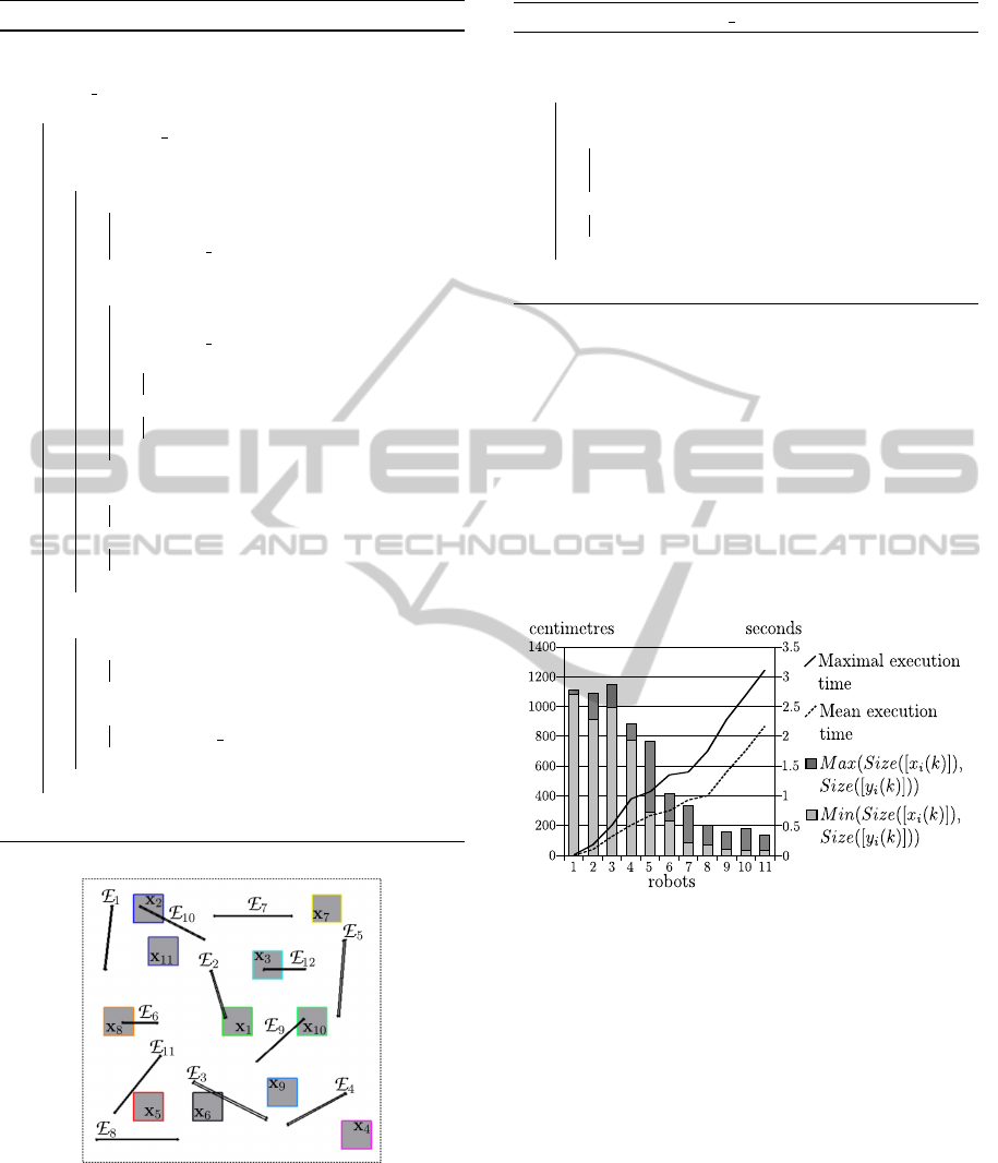
5.1 Influence of the Number of Robots
The objectiveit to evaluate the effect of the number of
robots for the localization. The considered environ-
ment is E =
6
S
j=1
E
j
. Figure 8 represents the obtained
results.
MobileRobotsPoseTracking-ASet-membershipApproachusingaVisibilityInformation
295

Algorithm 2: LUVIA algorithm.
Data: r
i
, y
i
, R , E
−
, E
+
1 L =
/
0, L
OK
=
/
0;
2 L .Push back([x
i
(k)]);
3 while L .Size() > 0 do
4 [x] = L .Pop out();
5 bisect = false;
6 for r
i
′
∈ R (with i 6= i
′
) do
7 if y
ii
′
= true then
8 consistent =
Visibility Test([x], [x
i
′
(k)], E
−
);
9 end
10 else
11 consistent =
Visibility Test([x], [x
i
′
(k)], E
+
);
12 if consistent = true then
13 consistent = false;
14 else if consistent = false then
15 consistent = true;
16 end
17 end
18 if consistent = false then
19 break;
20 else if consistent = indeterminate then
21 bisect = true;
22 end
23 end
24 if consistent 6= false then
25 if bisect = true and Size([x]) > ε then
26 Bisect([x], L );
27 end
28 else
29 L
O K
.Push back([x]);
30 end
31 end
32 end
Result: Hull(L
OK
).
Figure 7: The simulated environment. The black shapes
correspond to the environment E =
11
S
j=1
E
j
and the grey
boxes correspond to the initial boxes [x
i
(0)] of the robots
such as x
i
(0) ∈ [x
i
(0)], x
i
the initial position of the robot
r
i
∈ R , i = 1, ··· , 11. Note that for legibility reason E
+
and
E
−
are not represented. The doted lines do not represent
obstacles but robot’s move limits.
Algorithm 3: Visibility test.
Data: [x
1
], [x
2
], E
∗
1 visible = true;
2 for E
∗
k
∈ E
∗
do
3 inter = Intersect(Seg([x
1
], [x
2
]), E
∗
k
);
4 if inter < 0 then
5 visible = false;
6 break;
7 else if inter ≯ 0 then
8 visible = indeterminate;
9
10 end
Result: visible.
It appears that for a given environment a minimal
number of robots is necessary to perform an efficient
pose tracking. It can be explained by the fact that with
few robots, y
i
(k) carries few information. In this con-
figuration, at least 7 robots are necessary to perform
an efficient localization.
On the other hand, too many robots do not im-
prove significantly the localization but increase the
computation time. This localization maximal preci-
sion is directly dependent of E
−
and E
+
. In this ex-
ample, over 9 robots the results are similar.
Figure 8: Results over 1500 iterations.
5.2 Influence of the Number of
Obstacles
In this section the influence of the number of obstacles
over the localisation results is evaluated. A team of 7
robots is considered R = {r
i
}, i = 1, · ·· , 7. Figure 9
represents the obtained results.
It appears that for a given number of robots it ex-
ists a minimal and a maximal number of obstacles that
allow to perform an efficient localization. It can be
explained by the fact that without any obstacle, the
robots see each other all the time, so the visibility
sensor returns always the same value and does not
provide useful information. It is the same argument
with too many obstacles.
In Figure 9 it is possible to see that under 4 ob-
ICINCO2012-9thInternationalConferenceonInformaticsinControl,AutomationandRobotics
296

Figure 9: Results over 1500 iterations.
stacles and over 8 obstacles, the pose tracking does
not lead to an efficient localization of the robots. It
also appears that 7 obstacles do not lead to an efficient
pose tracking. Hence the success of the pose tracking
depends on the positions and the sizes of the obstacles
in the environment.
5.3 Conclusions
In this paper it is shown that using interval analysis it
is possible to perform a pose tracking of mobilerobots
even assuming weak informations as the visibility be-
tween robots. The LUVIA algorithm is a guaranteed
algorithm that exploits this boolean information.
It appears in Section 5.2 that characterizing the en-
vironments by counting the number of obstacles is not
pertinent here. In a future work it could be interest-
ing to characterize the environmentby visibility zones
allowing to calculate a minimal number of robots re-
quired to perform a pose tracking, according to the
number and/or the size of the zones.
Finally it could be interesting to process an exper-
imentation with actual robots.
REFERENCES
Abeles, P. (2011). Robust local localization for indoor en-
vironments with uneven floors and inaccurate maps.
In Intelligent Robots and Systems (IROS), 2011 IEEE/
RSJ International Conference on, pages 475 –481.
E. Seignez, M. Kieffer, A. L. E. W. T. M. (2005). Experi-
mental vehicle localization by bounded-error state es-
timation using interval analysis. In Intelligent Robots
and Systems, 2005. (IROS 2005). 2005 IEEE/RSJ In-
ternational Conference on, pages 1084 – 1089.
J. Borenstein, H. R. Everett, L. F. (1996). Navigating Mo-
bile Robots: Systems and Techniques. A. K. Peters,
Ltd.
J. Zhou, L. H. (2011). Experimental study on sensor fu-
sion to improve real time indoor localization of a mo-
bile robot. In Robotics, Automation and Mechatronics
(RAM), 2011 IEEE Conference on, pages 258 –263.
Jaulin, L. (2009). A nonlinear set membership approach
for the localization and map building of underwater
robots. Robotics, IEEE Transactions on, 25(1):88 –
98.
K. Lingemann, A. Nchter, J. H. H. S. (2005). High-speed
laser localization for mobile robots. Robotics and Au-
tonomous Systems, 51(4):275 – 296.
L. Jaulin, M. Kieffer, O. D. E. W. (2001). Applied Interval
Analysis. Springer.
M.J. Segura, V.A. Mut, H. P. (2009). Mobile robot self-
localization system using ir-uwb sensor in indoor en-
vironments. In Robotic and Sensors Environments,
2009. ROSE 2009. IEEE International Workshop on,
pages 29 –34.
Neumaier, A. (1991). Interval Methods for Systems of
Equations (Encyclopaedia of Mathematics and its Ap-
plications). Cambridge University Press.
P. Jensfelt, H. C. (2001). Pose tracking using laser scanning
and minimalistic environmental models. Robotics and
Automation, IEEE Transactions on, 17(2):138 –147.
R. E. Moore, R. B. Kearfott, M. J. C. (2009). Introduction
to Interval Analysis. SIAM.
APPENDIX
Segment Intersection
The function Intersect(), Definition 17, allows to test
the intersection between two segments.
Definition 17. Let Seg(x
1
, x
2
) and Seg(x
3
, x
4
) be two
segments, the function
Intersect(Seg(x
1
, x
2
), Seg(x
3
, x
4
)) (19)
is defined by
Intersect(Seg(x
1
, x
2
), Seg(x
3
, x
4
)) =
Max(Side(x
1
,Seg(x
3
, x
4
)) · Side(x
2
,Seg(x
3
, x
4
)),
Side(x
3
, Seg(x
1
, x
2
)) · Side(x
4
, Seg(x
1
, x
2
))).
where Side(), Definition 18, allows to test the side
of a point with a segment.
Definition 18. Let Seg(x
1
, x
2
) be a segment and x
3
be
a point, the function Side(x
3
, Seg(x
1
, x
2
)) is defined
by
Side(x
3
, Seg(x
1
, x
2
)) = det(x
3
− x
1
x
2
− x
1
), (20)
with det the determinant.
Figure 10 represents three intersection tests.
Figure 10: Three Intersect() tests.
MobileRobotsPoseTracking-ASet-membershipApproachusingaVisibilityInformation
297