Evaluation of a Joint Hysteresis Model in a Robot Actuated by

Pneumatic Muscles

Michael Kastner

, Hubert Gattringer

and Ronald Naderer

Institute for Robotics, Johannes Kepler University Linz, Altenberger Strasse 69, 4040 Linz, Austria

FerRobotics Compliant Robot Technology GmbH, Altenberger Strasse 69, 4040 Linz, Austria

Keywords:

Compliant Robotics, Pneumatic Muscles, Hysteresis Model.

Abstract:

Passively compliant drives are interesting alternatives to classical stiff actuators in emerging ﬁelds like human–

robot cooperation, service and rehabilitation robotics. Pneumatic muscles have been found to be interesting

low–cost actuators for such purposes. To fully realize the (desired) higher sensitivity and at the same time

maintain a good control quality, detailed models of the robot’s own components are required. For pneumatic

muscles, their hysteresis characteristic is a challenging property. In this paper we present a hysteresis model

based on a Prandtl–Ishlinskii operator approach and evaluate theresulting performance when the inverse model

is used for compensation in the position controller. The evaluation is done on a real multi–axes robot arm.

1 INTRODUCTION

Typical industrial robots are built as stiff as possi-

ble to ensure a high repeatability and tracking accu-

racy during free motion. For interaction tasks, the

use of compliant robotic systems has long been re-

searched. While this compliance is often added to

standard robots by means of additional control algo-

rithms and sensors, another approach is to use pas-

sively compliant drive technologies, i.e. actuators

with a low natural stiffness. Compliant actuation sys-

tems have been and are actively researched for a large

number of applications, including safe human/robot

interaction for industrial or service robotics, contact

processes, temporary energy storage, rehabilitation

devices and walking robots.

One type of actuation that is particularly inspired

by biological systems is the pneumatic muscle, which

was originally used by McKibben for prosthesis ap-

plications. It consists of a rubber tube and an inelas-

tic braided shell. When the tube is ﬁlled with pres-

surized air, the braid angle changes, causing a radial

expansion and a longitudinal contraction. Two such

muscles can be used in an antagonistic setup to create

a prismatic or revolute joint. Because of the low cost

of the muscle itself and the high forces it is able to

exert, its use in robotics has also been investigated by

several research groups.

Compared to pneumatic cylinders, the absence of

a stick–slip effect helps with an accurate position con-

trol, but the actuator characteristic is still very com-

plex and difﬁcult to handle. Particularly, hysteresis

causes disturbances every time the drive direction is

reversed, while a creep/settling characteristic causes

the actuation force to slowly drift after a maneuver.

In this paper we present a model for the hystere-

sis effect based on a Prandtl–Ishlinskii approach and

discuss its use as a compensation term in the position

controller of a pneumatically actuated industrial ma-

nipulator. Section 2 will detail the considered robot

and joint setup. In Section 3 we will discuss advanced

pneumatic muscle models that can be found in the lit-

erature and present our hysteresis model. The gen-

eral controlstructure used and the incorporation of the

hysteresis compensatorare shown in Section 4, before

measurement results from the real robot are presented

in Section 5. Section 6 closes with conclusions and

an outlook on planned activities.

2 SYSTEM SETUP

The robot system that we are dealing with in this

contribution is an industrial robot arm manufactured

by FerRobotics Compliant Robot Technology GmbH,

called Romo (see Figure 1). It comprises seven rota-

tional joints of which ﬁve are actuated pneumatically.

The other two – used for longitudinal rotations – are

driven by Schunk PowerCubes (electrically commu-

230

Kastner M., Gattringer H. and Naderer R..

Evaluation of a Joint Hysteresis Model in a Robot Actuated by Pneumatic Muscles.

DOI: 10.5220/0004024102300235

In Proceedings of the 9th International Conference on Informatics in Control, Automation and Robotics (ICINCO-2012), pages 230-235

ISBN: 978-989-8565-22-8

 2012 SCITEPRESS (Science and Technology Publications, Lda.)

Figure 1: Considered robot Romo with joints 1 to 7 and tool

(T) and base (B) coordinate systems.

tated motor modules). The three main joints (1, 2 and

4) are actuated by a pair of Festo DMSP–40 muscles

each. Only these three joints will be considered in this

paper. The basic joint principle is shown in Figure 2,

the controller will be presented later (see Figure 6).

q denotes the joint angle, Q the joint torque, F the

muscle forces, p the muscle pressures and u the valve

control voltages.

Each muscle pressure is measured by an according

sensor located at the inlet, while the robot’s original

joint position instrumentation has been changed from

cable extension sensors to optical encoders (17bit,

absolute) to improve the control performance. The

muscles are actuated by Festo MPYE–18HF 5/3-way

proportional directional slider valves. The control is

implemented on an industrial PC with a realtime op-

erating system (Bernecker and Rainer APC 620) with

a Pentium M CPU clocked at 1.4 GHz. The controller

cycle time is 0.5 ms. The Mathworks Realtime Work-

shop is used to generate C code for the PC from a

Simulink implementation of the controller, much like

on the well known dSpace rapid prototyping systems.

3 ADVANCED MUSCLE

MODELING

Beyond the static contraction/pressure/force charac-

teristic, several approaches for enhanced dynamical

models of pneumatic muscles can be found in various

publications. (Chou and Hannaford, 1994) observed

that the braided pneumatic muscles they used showed

a rate–independent hysteresis, which they attributed

to Coulomb friction in the shell or between the shell

and the bladder. They did not devise a mathematical

model but tried to improve the situation using lubri-

cants, which only led to small improvements. (Klute

Pressure

sensors

Position

sensor

Control

system

2 x

1 2

Tank

q, Q

Figure 2: Concept drawing of a pneumatic joint.

et al., 2002) from the same research group compared

the characteristic of the pneumatic artiﬁcial muscle

to the famous Hill model for skeletal muscle, (Hill,

1938). Again, they found the pneumatic muscle to be

very lightly damped and used an additional hydraulic

damper to create a mechanical system that resembles

the biological inspiration. The hysteresis effect is not

mentioned in this article. (Reynolds et al., 2003) de-

vise a model using spring and damper coefﬁcients that

are afﬁne functions in the muscle pressure. (Kerscher

et al., 2006) use a similar approach for modeling a

Festo ﬂuidic muscle. They evaluate their model in

a quick–release setup inspired by Hill’s experiments

and conclude that the resulting force/velocity charac-

teristic shows nearly the same curve progression as

biological muscle. Around the same time (Tondu and

Zagal, 2006) performed basically the same tests with

custom braided muscles. They show that a version

with a braided iron shell can be modeled with a con-

stant viscous friction coefﬁcient, while for a rayon

variant this constant has to be replaced by an ansatz

of the form a/(b+ v) (a and b are constant model pa-

rameters and v is the contraction speed). They demon-

strate that the latter resembles the behavior of biolog-

ical muscle, while the iron shell version leads to con-

siderably more oscillations. They also criticize (Klute

et al., 2002) for a misinterpretation of Hill’s model.

Again, none of the last three mentioned contribu-

tions consider hysteresis, although Tondu had used

Coulomb terms in older papers.

(Davis and Caldwell, 2006) took on ideas from

the already mentioned (Tondu and Lopez, 2000) and

(Chou and Hannaford, 1994) concerning Coulomb

friction to devise a very complex model of the braid’s

friction properties. Recently, (Minh et al., 2011)

presented a more phenomenological Maxwell–slip

model approach for single Festo MAS–20 muscles

EvaluationofaJointHysteresisModelinaRobotActuatedbyPneumaticMuscles

231

and the same was done for an antagonistic joint

in (Minh et al., 2010). They build on the rate–

independance assumption from the research group

around Hannaford and verify this assumption for the

Festo muscle. While this result is somewhat surpris-

ing when compared to the Hill’s model analogy previ-

ously found in (Kerscher et al., 2006) (who used ex-

actly the same muscle type), it seems that the main

reason for this discrepancy might be the different

considered speed ranges. For rotational joints the

arm transforms the muscle speed upwards to the tip.

Therefore, lower muscle speeds than in linear appli-

cations are typically used in such setups. While Minh

et al. use speeds of 1 mm/s and 16mm/s to support

their rate–independence assumption, the force/speed

characteristic by Kerscher et al. presumably

ranges

from 0 to 900mm/s.

(Minh et al., 2009) is the only contribution we

are aware of, where a hysteresis compensator is used

in a pneumatic muscle position controller and the

improvements are evaluated. (Boblan, 2009) pro-

vides some hysteresis modeling ideas for single Festo

muscles and also mentions that they are very lightly

damped. The lack of measurement data for the hys-

teresis behavior of the complete joint is given as a

reason for neglecting it in the control scheme. Sim-

ilarly, (Van Damme, 2009) develops a Preisach hys-

teresis model for pleated pneumatic artiﬁcial muscles

but states that without knowledge of the initial hys-

teresis state the utilization in a controller is too cum-

bersome. Other recent publications on position con-

trol, for example (Aschemann and Schindele, 2008)

or (Krichel et al., 2010) show a good controller per-

formance without explicitly considering effects like

hystersis, damping or friction in their models.

Here, we want to evaluate the usefulness of a local

compensator for the hysteresis in the joint angle for

quasi–static pressure differences. In our approach we

completely separate the nonlinear static characteristic

and the hysteresis model.

Our joint hysteresis model is based on a Prandtl–

Ishlinskii operator approach as described in (Kuhnen,

2003) for a magnetostrictive actuator. The nominal

pressure difference for a certain joint angle under the

zero load assumption, i.e. Q = 0, can be calculated

from the static joint model as

∆p

nom

B(q)

(−A(q) p

−C(q)) , (1)

where p

is the mean pressure and A, B and C are

polynomials that approximate pointwise, global (i.e.

In the referred to Figure 11 no explanation of the used

scaling value v

max

is given, so this assumption is based on

maximum speed values found in other plots.

(b)

(∆p− ∆p

nom

) + q

(a)

q in rad

∆p in bar

−1 0 1−2 0 2

−1

Figure 3: Hysteresis in the joint angle for slow variations

of ∆p (a). The nominal pressure difference was subtracted

and as a purely mathematical procedure the joint angle was

added to get a hysteresis loop around the 45

◦

line (b).

over the whole pressure/torque/angle range), calibra-

tion measurements. Additionally, we applied a local

calibration (i.e. for p

= 3bar and Q= 0) with a poly-

nomial ﬁt to really just extract the hysteresis cycle.

For the hysteresis parameter identiﬁcation pro-

cess we arranged the loop around the 45

◦

line by

adding the joint angle (in rad) to the difference be-

tween actualand nominal pressure differences (in bar)

as shown in Figure 3.

For the hysteresis model we adopted the nomen-

clature used in (Kuhnen, 2003). The output signal, y,

(which is q in our case) is directly the result of the

Prandtl–Ishlinskii operator,

y = H [x] = w

[x,z

] , (2)

which is a linear superposition, weighted by factors



H,1

H,2

... w

H,N



, (3)

of N elementary so–called play–operators,

[x,z

] =



H,1

[x,z

H0,1

] ...



, (4)

depending on the input signal, x, (∆p− ∆p

nom

+ q for

us) and the vector of initial internal states,



H0,1

H0,2

... z

H,N



. (5)

Like the vector of weights, the vector of thresholds,



0 r

H,2

... r

H,N



, (6)

is a parameter of the model.

The play operator (see Figure 4),

z = H

[x,z

] , (7)

is usually deﬁned recursively as

z = H (x,z,r

) (8)

with the initial condition



t=0

= z

(9)

ICINCO2012-9thInternationalConferenceonInformaticsinControl,AutomationandRobotics

232

and the threshold parameter r

∈ R

. Here,

H (x, z,r

) = max{x− r

,min{x+ r

,z}} (10)

is the sliding, symmetrical dead–zone function. For a

discrete time system, Equation 8 can be written as

= H (x

k−1

) (11)

with the index k denoting the k–th sample of a signal.

−r

0 r

Figure 4: Example input/output trajectory of the play oper-

ator, starting at an initial position z = 0. Note, that the slope

of the elementary operator is always 1.

To determine the parameters of the model, r

, z

and w

, we ﬁrst select evenly spaced threshold val-

ues,

H,i

i− 1

kxk

∞

, (12)

and initial states

H0,i

= 0 (13)

with i = 1..N. Then, the weights are calculated by

minimizing

J =

kek

dt, (14)

with the error

e = y− w

[x,z

] , (15)

subject to the inequality constraint

≥













, (16)

where ε is a positive, but arbitrarily small constant.

The time t

is the start and t

the end time of the mea-

sured hysteresis cycle (see Figure 3) towards which

the parameters are optimized.

For our application we chose N = 100 and ε =

0.001. We solved the quadratic optimization prob-

lem, Equations 14 and 16 for our time discrete mea-

surement data of x and y using the qpOASES package

from (Ferreau et al., 2008). Of the 100 weights only

14 turned out to be non–zero. Consequently, the ele-

mentary play operators associated with the remaining

weights were dropped for the ﬁnal model.

The inequality constraint, Equation 16, guarantees

an invertible model by limiting the slope of the hys-

teresis model to strictly positive values. The parame-

ters of the inverse operator,

−1

[y] = w

′



y,z

′



, (17)

can be calculated from

′

H,i

∑

j=1



H, j

H,i

− w

H, j

)



, (18)

′

H,i







H,1

i = 1

−

H,i



∑

j=1

H, j



∑

i−1

j=1

H, j



i = 2...N

and

(19)

′

H0,i

∑

j=1

H, j

H0,i

∑

j=i+1

H, j

H0, j

. (20)

Figure 5 shows a comparison of the inverse model

– corrected by the previously added q–term – to the

measurement data.

model output

measurement

q in rad

∆p− ∆p

nom

in bar

−1 −0.5 0 0.5 1

−0.2

0.2

0.4

0.6

0.8

Figure 5: Inverse hysteresis model output compared to mea-

surement data.

4 CONTROL

The implemented joint controllers (see Figure 6) use a

cascaded structure with inner, ﬂatness based, pressure

control loops. The position controller uses a PID con-

trol law for feedback and and additional feedforward

action from the inverse dynamics. A linear, local joint

observer estimates the states. It uses a nominal mo-

ment of inertia of the joint as model informationin ad-

dition to an integral estimation of the remaining load

torque components. A gain–scheduling anti–windup

logic has been added. However, it becomes only ac-

tive in case of fast and large disturbances, since our

target trajectories are designed to obey the actuator

ﬂow and pressure limits.

The calculated pressure difference of the compen-

sator is added to the output of the inv. joint character-

istic. Note, that for the ﬂatness based pressure control

the time derivative of the desired pressure is required,

which is generated by numerical differentiation.

EvaluationofaJointHysteresisModelinaRobotActuatedbyPneumaticMuscles

233

State observer

−

˙q

Anti-windup

logic

Inverse

dynamics

sensor

, p

d,1

, p

d,1

, u

d,1

, u

d,2

Q, p

, p

, u

−

m,d

Pressure

controller

, q

Pressure

controller

, q

d,1

d,2

d,1

d,2

ﬀ

Inv. joint

torque

character-

istic

, ˙q

, ¨q

Hysteresis

compensator

Figure 6: Implemented joint controller structure. Subscript d denotes desired values.

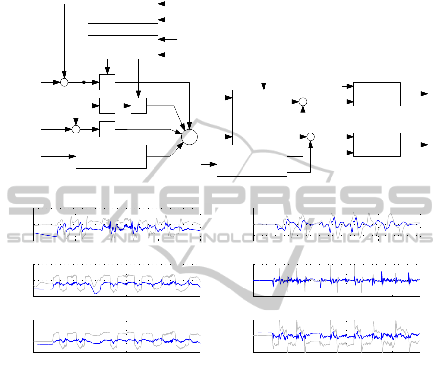
t in st in s

− q

1,d

in mrad

1,d

− Q

1,ff

in Nm

0 100 200 3000 100 200 300

100

200

300

0 100 200 300

0 10 20 30 400 10 20 30 40

−10

−20

−10

−20

Figure 7: Evaluation results of the hysteresis compensator for the ﬁrst joint of the Romo robot. Regular lines were taken with

enabled and light lines with disabled hysteresis compensator. The ﬁrst row is from the fast experiment while for the second a

time scaling of 1/10 was used. In the third the integrator part of the position controller was disabled for the slow experiment.

5 EVALUATION

The evaluation of the control performance when us-

ing the hysteresis compensator in the ﬁrst joint was

done tracking a trajectory designed to the recommen-

dations of the ISO 9283 norm (rounded rectangles,

cirles and lines in space) at different speeds. The re-

sults are shown in Figure 7. Especially in the slow

trial there is a signiﬁcant improvement in the control

quality. An interesting observation is that there seems

to be some interplay between the hysteresis compen-

sation and the integrator part of the controller – see

the difference in the torque errors at t = 130s where

the ﬁrst joint is at rest.

We have not yet created a hysteresis model for the

other two joints in the way described above. However,

in these joints the feedback part is working much bet-

ter than in the ﬁrst joint (see Figure 8, q

mainly in-

ﬂuences the y direction – see Figure 1).

6 CONCLUSIONS

In this paper we discussed the advanced modeling

of robot joints actuated by pneumatic muscles using

hysteresis compensation. We evaluated the result-

ing compensator in the position controller of a robot,

which led to promising results. In the future we want

to look into the observed interplay between the inte-

ICINCO2012-9thInternationalConferenceonInformaticsinControl,AutomationandRobotics

234

t in s

z− z

in mm

y− y

in mm

x− x

in mm

0 10

20 30 40

0 10 20 30 40

−10

Figure 8: Tracking errors during the fast ISO 9283 test with

(regular line) and without (light line) hysteresis compensa-

tion in the ﬁrst joint.

grator part and the hysteresis compensator as well as

devise models for the other joints. Furthermore, us-

ing the compensator in a disturbance force observer

would be an interesting scenario.

ACKNOWLEDGEMENTS

This work was supported by the Austrian Center

of Competence in Mechatronics (ACCM) and the

ODEUO project, an experiment funded in the context

of the European Clearing House for Open Robotics

Development (ECHORD) project.

REFERENCES

Aschemann, H. and Schindele, D. (2008). Sliding-mode

control of a high-speed linear axis driven by pneu-

matic muscle actuators. Industrial Electronics, IEEE

Transactions on, 55(11):3855–3864.

Boblan, I. (2009). Modellbildung und Regelung eines ﬂu-

idischen Muskelpaares. PhD thesis, Technical Univer-

sity Berlin.

Chou, C.-P. and Hannaford, B. (1994). Static and dynamic

characteristics of McKibben pneumatic artiﬁcial mus-

cles. In Robotics and Automation, 1994. Proceedings.,

1994 IEEE International Conference on, volume 1,

pages 281–286.

Davis, S. and Caldwell, D. G. (2006). Braid effects on con-

tractile range and friction modeling in pneumatic mus-

cle actuators. The International Journal of Robotics

Research, 25(4):359–369.

Ferreau, H., Bock, H., and Diehl, M. (2008). An online ac-

tive set strategy to overcome the limitations of explicit

MPC. International Journal of Robust and Nonlinear

Control, 18(8):816–830.

Hill, A. V. (1938). The heat of shortening and the dy-

namic constants of muscle. Proceedings of the Royal

Society of London. Series B, Biological Sciences,

126(843):136–195.

Kerscher, T., Albiez, J., Z¨ollner, J., and Dillmann, R.

(2006). Evaluation of the dynamic model of ﬂuidic

muscles using quick-release. First IEEE / RAS-EMBS

International Conference on Biomedical Robotics and

Biomechatronics.

Klute, G. K., Czerniecki, J. M., and Hannaford, B. (2002).

Artiﬁcial muscles: Actuators for biorobotic sys-

tems. The International Journal of Robotics Research,

21(4):295–309.

Krichel, S., Sawodny, O., and Hildebrandt, A. (2010).

Tracking control of a pneumatic muscle actuator us-

ing one servovalve. In American Control Conference

(ACC), 2010, pages 4385–4390.

Kuhnen, K. (2003). Modeling, identiﬁcation and compen-

sation of complex hysteretic nonlinearities: A modi-

ﬁed Prandtl-Ishlinskii approach. European Journal of

Control, 9:407–418.

Minh, T., Tjahjowidodo, T., Ramon, H., and Van Brussel,

H. (2009). Control of a pneumatic artiﬁcial mus-

cle (PAM) with model-based hysteresis compensa-

tion. In Advanced Intelligent Mechatronics, 2009.

AIM 2009. IEEE/ASME International Conference on,

pages 1082–1087.

Minh, T. V., Kamers, B., Tjahjowidodo, T., Ramon, H.,

and Van Brussel, H. (2010). Modeling torque-

angle hysteresis in a pneumatic muscle manipula-

tor. In Advanced Intelligent Mechatronics (AIM),

2010 IEEE/ASME International Conference on, pages

1122–1127.

Minh, T. V., Tjahjowidodo, T., Ramon, H., and Van Brussel,

H. (2011). A new approach to modeling hysteresis in

a pneumatic artiﬁcial muscle using the Maxwell-slip

model. Mechatronics, IEEE/ASME Transactions on,

16(1):177–186.

Reynolds, D. B., Repperger, D. W., Phillips, C. A., and

Bandry, G. (2003). Modeling the dynamic character-

istics of pneumatic muscle. Annals of Biomedical En-

gineering, 31:310–317.

Tondu, B. and Lopez, P. (2000). Modeling and control of

McKibben artiﬁcial muscle robot actuators. Control

Systems, IEEE, 20(2):15–38.

Tondu, B. and Zagal, S. (2006). McKibben artiﬁcial mus-

cle can be in accordance with the Hill skeletal muscle

model. In Biomedical Robotics and Biomechatronics,

2006. BioRob 2006. The First IEEE/RAS-EMBS Inter-

national Conference on, pages 714–720.

Van Damme, M. (2009). Towards Safe Control of a Com-

pliant Manipulator Powered by Pneumatic Muscles.

PhD thesis, Vrije Universiteit Brussel.

EvaluationofaJointHysteresisModelinaRobotActuatedbyPneumaticMuscles

235