A Generative Traversability Model for Monocular Robot Self-guidance

Michael Sapienza and Kenneth P. Camilleri

Department of Systems & Control Engineering, University of Malta, Msida MSD 2080, Malta

Keywords:

Traversability Detection, Autonomous Robotics, Self-guidance.

Abstract:

In order for robots to be integrated into human active spaces and perform useful tasks, they must be capa-

ble of discriminating between traversable surfaces and obstacle regions in their surrounding environment. In

this work, a principled semi-supervised (EM) framework is presented for the detection of traversable image

regions for use on a low-cost monocular mobile robot. We propose a novel generative model for the occur-

rence of traversability cues, which are a measure of dissimilarity between safe-window and image superpixel

features. Our classiﬁcation results on both indoor and outdoor images sequences demonstrate its generality

and adaptability to multiple environments through the online learning of an exponential mixture model. We

show that this appearance-based vision framework is robust and can quickly and accurately estimate the prob-

abilistic traversability of an image using no temporal information. Moreover, the reduction in safe-window

size as compared to the state-of-the-art enables a self-guided monocular robot to roam in closer proximity of

obstacles.

1 INTRODUCTION

Giving autonomous robots the ability to explore

and navigate through their environment using

CCD/CMOS cameras has become a major area in

mobile robotics research (DeSouza and Kak, 2002).

This paper addresses the fundamental problem of de-

termining terrain traversability for a mobile robot

equipped with a single camera (Lorigo et al., 1997;

Ulrich and Nourbakhsh, 2000; Santosh et al., 2008;

Katramados et al., 2009).

Even though autonomous guidance has achieved

relative success using active sensors, this task still

remains challenging for robots equipped with vision

sensors (Santosh et al., 2008). However, in addition

to providing local depth information in the vicinity

of the robot, camera information has the potential to

provide long-range traversability information and en-

vironmental semantics (Hadsell et al., 2009; Hoiem

et al., 2007), making it ideal for mobile robot explo-

ration and navigation.

Multiple camera vision has been used for depth

estimation and image analysis (Roning et al., 1990),

however in practice, 3D reconstruction works well for

close objects, with the accuracy diminishing signiﬁ-

cantly with distance from the camera (Michels et al.,

2005; Hadsell et al., 2009). Recent self-guided vehi-

cles used in the DARPA LAGR programme have led

to signiﬁcant advances in robotic perception systems

(Hadsell et al., 2009; Sofman et al., 2006; Kim et al.,

2007), however the multiple sensors and complexity

of these systems do not address the needs of low-cost

autonomous robots (Katramados et al., 2009; Murali

and Birchﬁeld, 2008). A commonly available web

camera presents a desirable alternative that will be

used in this work, and is motivated by the human abil-

ity to interpret 2D low resolution images (Murali and

Birchﬁeld, 2008).

A self-guided monocular robot needs to extract in-

formation on surrounding objects in order to identify

areas through which it can move. This problem has

been approached by providing the robot with a de-

tailed description of its environment, usually an ex-

plicit geometric or topological map built manually or

extracted from the stereo/monocular vision sensors on

the robot (Kosaka and Kak, 1992; Meng and Kak,

1993; Ohno et al., 1996). Building such representa-

tions of the environment is time-consuming, and con-

strains the limits of operation of the robot to the par-

ticular environment in which the hard-data was col-

lected. For mobile robots that can be used in dynam-

ically changing environments, a basic form of scene

traversability understanding must be available to the

robot (Kim et al., 2007). This computer vision task

forms a basic building block that intelligent systems

will need to gain autonomy, and upon which more

complex behaviours can be built.

Motivated by autonomous Martian landscape ex-

177

Sapienza M. and Camilleri K..

A Generative Traversability Model for Monocular Robot Self-guidance.

DOI: 10.5220/0003983701770184

In Proceedings of the 9th International Conference on Informatics in Control, Automation and Robotics (ICINCO-2012), pages 177-184

ISBN: 978-989-8565-22-8

 2012 SCITEPRESS (Science and Technology Publications, Lda.)

ploration, Lorigo (Lorigo et al., 1997) proposed an

appearance-based approach to traversability detection

in which a rectangular safe-window of pixels towards

the bottom of the captured image is assumed to be

traversable. This appearance-based technique was

shown to work in real-time and was implemented in

various indoor (Ulrich and Nourbakhsh, 2000; San-

tosh et al., 2008), and outdoor (Lorigo et al., 1997;

Katramados et al., 2009) environments. The size of

the safe-window determines the closest safe distance

between the robot and obstacles, for a given camera

pose and optical properties. Thus, a smaller safe-

window will allow greater robot agility and manoeu-

vrability between obstacles in a cluttered environ-

ment. Moreover, reducing the size of the safe-window

allows dynamic obstacles to move closer to the robot

without the risk of being captured in this window.

Due to the real-time requirement of mobile robotic

systems, image region classiﬁcation must be compu-

tationally efﬁcient. Ulrich (Ulrich and Nourbakhsh,

2000) used a static threshold on the feature his-

tograms of the safe-window pixels to determine im-

age traversability, making this approach unsuitable

for other novel environments that may require differ-

ent thresholds. Santosh (Santosh et al., 2008) based

his method on that of Ulrich stating that the his-

togram threshold is determined from the histogram

entropy, but does not provide any details how this is

achieved. On the other hand, Katramados (Katrama-

dos et al., 2009) determines a classiﬁcation threshold

from the safe-window histogram peak and mean level,

thus clearly showing that the classiﬁcation method al-

lows the robot to be used in other novel environments.

However, a histogram with multiple peaks may result

from a safe-window over composite surfaces, thereby

employing multiple thresholds. An interesting simpli-

ﬁed alternative is proposed by Lorigo (Lorigo et al.,

1997), where the area of overlap between the feature

histograms of the safe window and that of rectangu-

lar patches is computed. However a static threshold

on this area is used to assign a traversable or non-

traversable label to each image patch, making it un-

suitable to novel environments without threshold tun-

ing. In this work, we develop a framework that al-

lows the robot to be used in novel environments, as

in (Katramados et al., 2009), and that uses a dis-

similarity measure between image regions as a cue

for traversability, as in (Lorigo et al., 1997). How-

ever, instead of using the feature distributions directly

(Lorigo et al., 1997; Ulrich and Nourbakhsh, 2000;

Santosh et al., 2008; Katramados et al., 2009), we

propose to model the feature dissimilarity distribu-

tion. This allows a probabilistic framework to be used

in which the dissimilarity model parameters are self-

learned in a semi-supervised manner, allowing the

robot to be used in new environments.

The main contribution of this work is a novel gen-

erative model for the classiﬁcation of traversable im-

age regions with the safe-window approach (cf. Sec-

tion 2.5). In addition to the inherent environment

adaptability provided by the safe-window (Lorigo

et al., 1997; Ulrich and Nourbakhsh, 2000; Santosh

et al., 2008; Katramados et al., 2009), our traversabil-

ity classiﬁcation method (cf. Section 2) is based

upon a principled framework in which a mobile robot

can also self-learn its model parameters in any novel

environment where the traversable region differs by

some degree to the appearance of obstacles. Simi-

larly to previous safe-window approaches, once the

robot is initialized in a particular environment, it

cannot make a transition to another traversable sur-

face with different appearance properties, unless the

safe-window is reinitialized manually or automati-

cally by means of active sensors. Once initialized

however, our method will allow the model parame-

ters to adapt to the present ground/obstacle dissimi-

larity and varying lighting conditions of the ground

in a semi-supervised manner. In the experimental

section (cf. Section 3) we demonstrate that our ap-

proach allows robust traversability classiﬁcation on

single image frames without requiring temporal in-

formation (cf. Section 3.1). This means that the al-

gorithm may be used intermittently alongside other

computationally intensive algorithms such as human

gesture recognition. Furthermore, the method is ro-

bust to the reduction in safe-window size, without loss

in classiﬁcation performance (cf. Section 3.2). This

allows a mobile robot to guide-itself safely and ma-

neuver in a tight corridor space cluttered with obsta-

cles (cf. Section 3.3).

2 METHODS

In this work, traversability detection is accomplished

by adopting the well-known principled probabilistic

framework based on Bayes’ rule to infer the class la-

bel of image regions from traversability cues. The

traversability cues X = hX

, X

, ...X

i are found

by comparing descriptive feature distributions (cf.

Section 2.1) from oversegmented regions called su-

perpixels (cf. Section 2.2) to those in the safe-

window, by using a dissimilarity metric (cf. Sec-

tion 2.3). Initially, n descriptive feature distributions

and h

, where j = 1, ..., n, are extracted from im-

age superpixel S and from the safe-window M re-

spectively, as illustrated in Fig. 1. The traversabil-

ity cue values X

= x

= d(h

) are a measure of

ICINCO2012-9thInternationalConferenceonInformaticsinControl,AutomationandRobotics

178

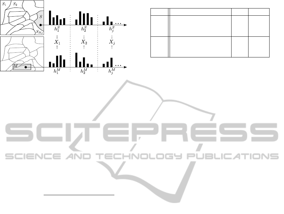
Figure 1: The discrete distributions of the descriptive fea-

tures in each superpixel S are compared to those of the

model in M. For each traversability cue j, a random variable

is found by comparing the query and model distributions

with a dissimilarity metric.

dissimilarity between the descriptive feature distribu-

tions in S and M. The occurrence of traversability

cue values are modelled by a generative traversability

model (cf. Section 2.5), whose parameters are up-

dated from the traversability cue statistics by means

of the Expectation-Maximization algorithm (cf. Sec-

tion 2.6). Finally, Bayes’ rule is used to calculate

the posterior probability P(Θ|X) of a superpixel be-

ing traversable, given a vector of traversability cues

P(Θ = θ

|X) =

P(X|Θ = θ

)P(Θ = θ

)

∑

P(X|Θ = θ

)P(Θ = θ

)

, (1)

where Θ = θ

is a Boolean random variable repre-

senting the l

class label of superpixel S, and which

can take on values deﬁned by Θ ∈ {θ

, θ

}. In this

case, θ

and θ

represent the traversable and non-

traversable classes respectively.

Assuming conditional independence between

traversability cues X

, the most likely class label is

chosen using the maximum a posteriori (MAP) deci-

sion rule by

∗

← argmax

P(Θ = θ

)

∏

j=1

P(X

|Θ = θ

). (2)

Note that this probabilistic framework allows a

high degree of ﬂexibility in the choice of descrip-

tive features, image primitives, comparison metrics,

prior, and modelling of the traversability cue values.

Though it is not the purpose of this work to com-

pare different techniques in various stages of the algo-

rithm, this framework affords a straightforward way

to do so. The following subsections will describe the

design choices for each element of the framework.

2.1 Descriptive Features

The set of descriptive features that are considered in

this work were inspired from (Lorigo et al., 1997; Ul-

Table 1: Descriptive Features.

No. j Features Dim. Type

1 Hue colour channel 32

Colour

2 Saturation colour channel 32

3 Illumination Invariant Channel 32

4 Edge gradient magnitudes 32

Texture

5 Edge gradient orientations 9

6 Local Binary Patterns (LBP) 32

rich and Nourbakhsh, 2000; Katramados et al., 2009;

Davidson and Hutchinson, 2003), and are listed in

Table 1. The colour features have been chosen to

minimize the effects of shadows and reﬂections that

can confuse the classiﬁer (Katramados et al., 2009;

Ulrich and Nourbakhsh, 2000; Lorigo et al., 1997).

The three illumination invariant colour cues consid-

ered are the hue (H) and Saturation (S) channels of

the HSV colour space, and a combination of intensity

invariant channels from the YCbCr and LAB colour

space. This Illumination Invariant Colour channel is

found by a weighted combination of the Cb, Cr, and A

colour channels, as suggested by (Katramados et al.,

2009).

Texture features are also important where colour

information is not sufﬁcient or even present at all. We

consider the edge gradient magnitudes and orienta-

tions as is common in object recognition (Dalal and

Triggs, 2005), and the local texture distributions pro-

vided by the Local Binary Pattern Operator (LBP),

which can be computed very efﬁciently (Davidson

and Hutchinson, 2003; M

aenp

a et al., 2003).

2.2 Oversegmentation

The basic image regions used for traversability classi-

ﬁcation have classically been pixels (Ulrich and Nour-

bakhsh, 2000; Katramados et al., 2009) or rectangular

patches (Lorigo et al., 1997). Using pixels may re-

sult in a noisy/spotty classiﬁcation since pixel neigh-

bourhoods are not considered. Patch based classiﬁca-

tion allows local feature distributions to be extracted,

but may contain multiple object boundaries within

the same region. An oversegmented representation of

the image into superpixels overcomes these shortcom-

ings since superpixels delineate homogeneous pixel

regions whilst preserving the image structure. Thus

rich pixel statistics can be extracted from more per-

ceptually meaningful regions (Kim et al., 2007; San-

tosh et al., 2008; Hoiem et al., 2007).

In this implementation, the initial pixel group-

ing is done using the fast oversegmentation tech-

nique from (Felzenszwalb and Huttenlocher, 2004).

We have used the code publicly released by the au-

thors with the parameters σ = 0.5, k = 100, min =

AGenerativeTraversabilityModelforMonocularRobotSelf-guidance

179

100, where σ is a smoothing constant, k is a thresh-

old which determines how readily image regions are

joined together, and min is minimum superpixel size

(Hoiem et al., 2007).

2.3 Dissimilarity Metric

In the current implementation, the dissimilarity mea-

sure used to compare the superpixel and safe-window

feature distributions is the G-statistic. This dissimi-

larity measure is based on the Kullback–Leibler cross

entropy measure, and was inspired from (M

aenp

et al., 2003) where it was used to compare the dis-

tributions of local binary patterns.

2.4 Simple Prior

Using the exponential function, a heuristic prior is

constructed which favours superpixels towards the

lower parts of the image to be traversable. Let

the prior likelihood functions for the expectation of

traversable superpixels before seeing the data be ex-

ponentially distributed with rate λ:

P(C|θ

) =

−λC

, P(C|θ

) =



1 −e

−λC



(3)

Thus, the probability of a superpixel being

traversable given its centre pixel row position C (the

mean superpixel pixel height in the image) may be ex-

pressed by the following equation from Bayes’ rule:

P(Θ = θ

|C) =

1 +

λC

− 1)

, (4)

where Y

and Y

are normalization values updated on

each iteration to ensure the probability over all pos-

sible height values sums to one. The rate parameter

λ fully describes the exponential distribution, and its

Maximum Likelihood Estimate (MLE)

λ is the recip-

rocal of the sample mean

C of traversable superpixels

(Garthwaite et al., 2002).

2.5 Generative Traversability Model

The superpixels S in image I originate from either the

traversable (θ

) or non-traversable (θ

) class. Since

the safe-window M is a priori traversable, when it is

compared to a traversable superpixel, a low dissim-

ilarity is expected (approaching zero). On the other

hand, if the safe window is compared to a superpixel

from the non-traversable class, a large dissimilarity

score is expected (approaching a maximum g

max

However, it is also possible to have obstacle regions

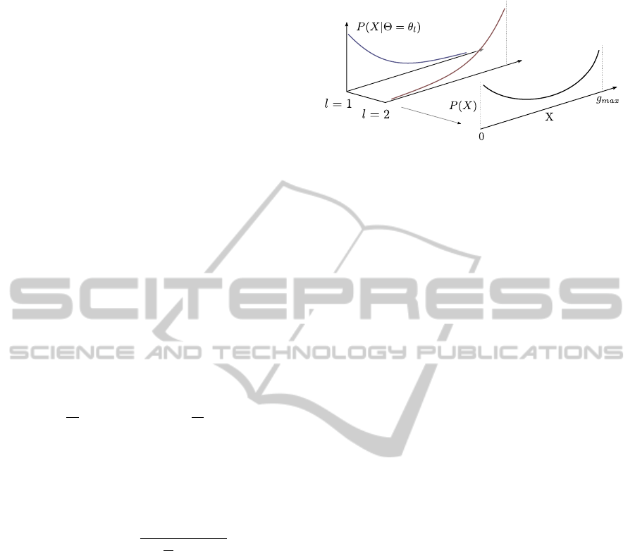
Figure 2: Mixture of two truncated exponential distribu-

tions. The mixture density created by marginalizing over

the hidden variable l, which acts as an identiﬁer for each

truncated exponential distribution.

similar in appearance to the ground, although with a

lower probability. This reasoning can be captured in a

generative model in which the probability of a random

traversability cue X

is a mixture of two truncated ex-

ponential distributions, as shown in Fig. 2.

The likelihood functions for the random variable

, given it was generated by matching a superpixel

from class label θ

to the safe-window M is a (one-

sided) truncated exponential which can be expressed

P(X

|θ

) = α

−α



1 − e

−α

max



−1

, (5)

P(X

|θ

) = α

max

− 1)

−1

, (6)

where 0 ≤ X

≤ g

max

, and α

> 0 is the rate parameter

of the distribution. The rate parameters need to be

learned from the data and this is achieved using the

EM algorithm which is discussed next.

2.6 Expectation Maximization (EM)

The learning task required here is to output a hypoth-

esis h

= hα

, α

i for each traversability cue j, that

describes the rate parameters of the exponential mix-

ture. Since it is not known which distribution gave

rise to the current observation, the EM algorithm will

be used to iteratively re-estimate the parameters given

some current hypothesis:

E-Step. Calculate the expected value E[θ

, h

] that

the l

truncated exponential distribution was respon-

sible for the j

traversability cue originating from su-

perpixel k, assuming h

holds. We will denote this

responsibility by r

M-Step. Calculate the new maximum likelihood hy-

pothesis h

[t+1]

= hα

[t+1]

, α

[t+1]

i assuming that the val-

ues for the responsibility r

were those calculated

from Step 1.

It can be shown that the maximum likeli-

hood estimate for a single exponential distribution

parametrized by α

given the observed data instances

ICINCO2012-9thInternationalConferenceonInformaticsinControl,AutomationandRobotics

180

Table 2: Safe window dimensions used by various authors.

Author Shape Dimensions % Area

Our Model Rectangular

4.2

Katramados Rectangular

12.5

Lorigo Rectangular

3.2

6.4

15.6

Ulrich Trapezoidal a =

, b =

, h =

3.3

22.3

, x

, ...x

i is the reciprocal of the sample

mean (Garthwaite et al., 2002):

[t+1]

¯x

[t+1]

, where ¯x

[t+1]

∑

, (7)

and |S

| is the size of superpixel S

in pixels (k =

1, ..., N

). This expression is a weighted sample mean

of x

, where each instance is weighted by the expected

value that it was generated by one of the two exponen-

tial distributions (Mitchell, 1997; Prince, 2011). Note

that since the exponential distribution is truncated, the

mean of the distribution becomes

¯x

− g

max



max

− 1



−1

, where

¯x

(8)

and

will be a MLE only if 0 < ¯x

max

(Al-

Athari, 2008).

3 EXPERIMENTAL RESULTS &

DISCUSSION

In order to test the validity of our approach, the vi-

sion framework was tested on three datasets: i) a

Static Traversability dataset containing still images,

ii) the Cranﬁeld University dataset containing video

sequences acquired from a teleoperated robot (Katra-

mados et al., 2009), and iii) a Self-Guided dataset

captured from a low-quality webcam during robot

autonomous guidance. All images were reduced to

a resolution of 160 × 120 and the size of the safe-

window was set to:

, whose top left corner is lo-

cated at position

, where W , H are the width and

height of the image respectively. The various safe-

window sizes used in the literature are compared in

Table 2.

3.1 Static Traversability Dataset

This dataset is made up of 100 challenging images

of indoor and outdoor scenes picked from the Inter-

net. These images contain scenes with highly reﬂec-

tive surfaces, specular reﬂections and traversable re-

gions with varying amount of colour and texture, as

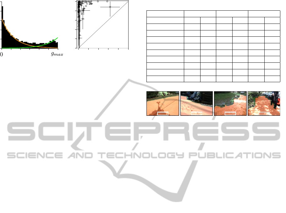
Figure 3: A sample of surfaces classiﬁed in the Static

Traversability dataset including indoor tiling, dirt roads,

textured carpets and wet roads with specular reﬂections.

The red highlighted area shows the accessible traversable

region. The white box towards the bottom of the image de-

notes the position of the safe-window.

shown in Fig. 3. Ground truth information was ob-

tained through manual labelling of the traversable im-

age regions by a human observer, and is made avail-

able online

3.1.1 Generative Model Validation

In this experiment, the traversability cues obtained

from the 100 images in the Static Traversability

dataset are accumulated in a histogram, shown in

Fig. 4(a). The shape of the histogram shows that the

distribution of the traversability cues X can in fact be

modelled as the joint mixture of two truncated expo-

nential distributions and demonstrates the suitability

of our proposed generative traversability model.

3.1.2 Image Classiﬁcation & EM Initialization

Sensitivity

The objective of this experiment was to test the ac-

curacy of traversability classiﬁcation on images from

multiple scenes with no temporal information. Each

test image was subjected to 100 random initializations

where the rate parameters α

and truncation point

max

were randomly initialized to values within the

range [0.01 - 10.01]. The algorithm was allowed to

iterate until the parameters converged, or up to a max-

imum of 10 iterations.

The mean TPR and FPR obtained for each im-

age, together with one standard deviation is shown

in Fig. 4(b). Images which always converged to

the same result have zero standard deviation. Those

points with a large cross-size resulted from images

which converged to different TPR-FPR results. Over-

all, 89% of the images converged to 1 - 2 identical

FPR-TPR values, and the mean classiﬁcation accu-

racy was 91.62% with a standard deviation of 8.78%.

The model parameters α

typically converged within

3-5 iterations, with respective processing times vary-

ing from 80-150ms. This result demonstrates the

model robustness to random initialization, and the

adaptability of its classiﬁcation model parameters to

multiple types of indoor and outdoor environments

Visit: https://sites.google.com/site/mikesapi

AGenerativeTraversabilityModelforMonocularRobotSelf-guidance

181

(a)

0.0 0.2 0.4 0.6 0.8 1.0

False positive rate

True positive rate

(b)

Figure 4: (a) Histogram of normalized traversability cues X

accumulated from the Static Traversability dataset, which

demonstrates the suitability of our generative traversability

model (cf. Section 2.5). (b) ROC plot showing the mean

and one standard deviation resulting from the static image

classiﬁcation.

with no temporal model, in contrast to (Katramados

et al., 2009) which uses a temporal memory model.

Note that the output of our algorithm can be extended

by a tracking algorithm which incorporates tempo-

ral and kinematic information. Errors occurred where

more than one ground type was present in the image,

of which one was not represented in the safe-window,

and when obstacle regions had a similar appearance

to the ground.

3.2 Cranﬁeld University Dataset

This dataset provided by Katramados et al. (Katra-

mados et al., 2009), consists of eight outdoor video

sequences captured from a teleoperated mobile robot.

Ground truth labelling was available from the author

at a rate of one frame per second. The video se-

quences were captured over a wide range of outdoor

conditions (cloudy, wet, sunny, shadows), and a range

of terrain types (concrete, grass, soil, tarmac, snow),

as shown in Fig. 5.

This experiment shows that our method can easily

be extended to video sequences and operate in real-

time. Instead of allowing the EM algorithm to con-

verge on each video frame (cf. Section 3.1.2), the cor-

relation between frames allows the algorithm to con-

verge across frames. This reduces the computational

cost to 30-50ms on each image (20-30fps). The accu-

racy results obtained using a 12.5% area safe-window,

a 4.2% area safe-window, and the result Safe-4.2|25 of

discarding 24 out of 25 frames in each sequence are

listed in Table 3. The similar results from Safe-12.5%

and Safe-4.2% demonstrate that the reduction in safe-

window size from 12.5% to just 4.2% of the image

area did not reduce the accuracy of the algorithm.

This makes it more suitable for self-guided robots to

move about in the proximity of obstacles, as detailed

in the Self-guided experiment. The ROC plots for the

4.2% area safe-window results are shown in Fig. 6,

Table 3: Cranﬁeld University dataset results.

Safe-12.5% Safe-4.2% Safe-4.2|25

Conditions %Acc %Std %Acc %Std %Acc %Std

Cloudy Dry 95.11 2.11 95.35 2.57 94.91 4.40

Cloudy Wet 93.54 3.94 93.74 4.53 92.15 11.12

Cloudy Muddy 91.63 4.00 89.30 6.62 81.49 15.28

Sunny Wet 82.13 9.49 82.32 8.88 71.24 12.71

Complex Shadow 83.98 9.10 85.77 6.35 85.20 8.46

Sunny Dry 89.64 4.61 89.71 4.53 84.73 13.99

Strong Shadows 85.23 15.62 88.33 12.42 87.03 14.39

Snow 88.50 10.95 89.19 10.29 89.18 9.93

Mean 88.72 7.48 89.21 7.02 85.74 11.29

Figure 5: Sample images of the classiﬁcation results taken

from the Cranﬁeld University dataset. The samples were

taken from videos (starting from left): Strong Shadows,

Snow, Cloudy Muddy, Cloudy Wet, Complex Shadows.

where it is seen that our model achieves better perfor-

mance in environments where the ground and obsta-

cles have a contrasting appearance (e.g. Cloudy Dry,

Cloudy Wet, Sunny Dry, Snow), than environments

where the ground obstacle boundary is not easily dis-

criminable (e.g. Cloudy Muddy, Sunny Wet). Drop-

ping 24 out of 25 frames in each video sequence, the

accuracy results in Safe-4.2%|25 were negatively af-

fected, more so in Sunny Wet where the appearance of

the ground is changing very quickly. In the other se-

quences however, this robustness makes it possible to

use the traversability algorithm intermittently along-

side other computationally expensive algorithms. Al-

though the authors of the dataset (Katramados et al.,

2009) reported higher classiﬁcation rates (97.6% Acc,

2.7% Std) on these video sequences, Katramados et

al. included a temporal model in their framework,

thus a direct comparison of the results is not possible.

The results in (Katramados et al., 2009) are given for

ofﬂine classiﬁcation; in the next sub-section we pro-

vide performance results for online autonomous robot

self-guidance, which is the ultimate purpose of this

system.

3.3 Self-guided Dataset

An experiment was set up in which our ERA-MOBI

mobile robotic platform named VISAR01 was placed

in a previously unknown indoor corridor environment

cluttered with a variety of objects typically found in-

doors: a chair, plant, box, waist paper basket, tool

box, and a person standing in the way. The ﬂoor

tiles are a pale grey, making them difﬁcult to dis-

ICINCO2012-9thInternationalConferenceonInformaticsinControl,AutomationandRobotics

182

−12

−8

−4

Cloudy Dry

True positive rate

0.0 0.2 0.4 0.6 0.8 1.0

−12

−8

−4

Cloudy Wet

True positive rate

0.0 0.2 0.4 0.6 0.8 1.0

−12

−8

−4

Cloudy Muddy

−12

−8

−4

Sunny Wet

−12

−8

−4

Complex Shadows

−12

−8

−4

Sunny Dry

False positive rate

0.0 0.2 0.4 0.6 0.8 1.0

−12

−8

−4

Strong Shadows

−12

−8

−4

Snow

False positive rate

0.0 0.2 0.4 0.6 0.8 1.0

True positive rate

0.0 0.2 0.4 0.6 0.8 1.0

True positive rate

0.0 0.2 0.4 0.6 0.8 1.0

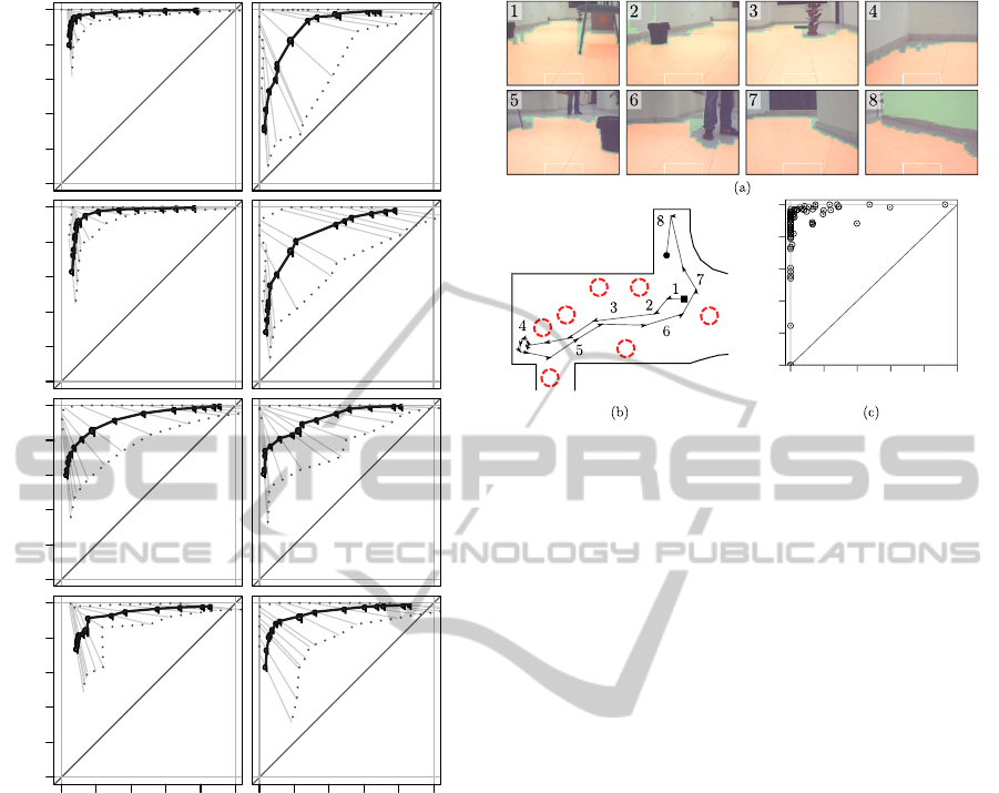
Figure 6: Mean ROC (black dots) and one standard devia-

tion (grey lines) for the classiﬁcation of video sequences in

the Cranﬁeld University dataset. The curves were plotted

by varying the log posterior ratio at which classiﬁcation is

decided.

tinguish from the white, untextured wall. In this ex-

periment, the horizon boundary that results from the

classiﬁcation was used to steer the robot towards the

largest open space (Santosh et al., 2008). The robot

moved at 0.15m/sec and the algorithm was run on ev-

ery frame at 25 fps. A video frame from the camera

together with its corresponding on-line classiﬁcation

result was saved every 25

frame, for a total of 99

frames in the 99 second sequence. Ground truth data

was collected by asking a human observer to man-

ually label the image regions as traversable or non-

traversable.

A sample of the resulting traversability classiﬁca-

tion and the path taken by the robot during the au-

tonomous movement can be seen in Fig. 7a&b. The

resulting ROC scatter plot is shown in Fig. 7c. Over-

0.0 0.2 0.4 0.6 0.8 1.0

False positive rate

True positive rate

Figure 7: (a) Samples image results from the Self-Guided

dataset. (b) Illustration of path taken by the robot moving

autonomously through a faculty corridor dotted with static

obstacles (dashed red circles). (c) ROC scatter plot for the

traversable ground classiﬁcation during self-guidance.

all, the mean and standard deviation of the classiﬁ-

cation accuracy for this successful run were 89.71%

and 9.68% respectively. The low levels of colour and

texture in this sequence made the ﬂoor and wall in-

distinguishable at times, however when the robot ap-

proached an obstacle their difference to the ground

became more apparent and therefore this did not con-

fuse the motion of the robot. Despite a high but im-

perfect classiﬁcation accuracy, the robot successfully

managed its way around the corridor and obstacles us-

ing only a monocular web-camera and turned back on

itself when it encountered a dead-end. As the ground

appearance changes gradually due to changing light-

ing and reﬂections, the classiﬁcation model was able

to adapt to these changes. The robot may transit to

a surface with different appearance characteristics by

re-initializing the traversability model and allowing

new model parameters to be self-learned.

4 CONCLUSIONS AND FUTURE

WORK

A real-time vision algorithm has been designed for

a mobile robotic platform to detect traversable ar-

eas and guide itself safely in proximity of obstacles

using the smallest reported safe-window. We have

modelled the feature dissimilarity distribution with a

truncated exponential mixture model and showed the

model’s competence without the need for a tempo-

ral model, prior training, or manual adjustments to

AGenerativeTraversabilityModelforMonocularRobotSelf-guidance

183

the system parametrization. The robustness of the

generative model to initialization, and its ability to

learn the model parameters for textured/untextured,

indoor/outdoor environments have been demonstrated

through experimental analysis and from the many

hours VISAR01 has been allowed to roam out into

the faculty corridors, avoiding both static and dy-

namic objects.

Future work will see the inclusion of structure-

from-motion depth estimation to allow the robot to

transition from one type of surface to another auto-

matically, and new exploration behaviours based on

the probability of traversability, rather than simple bi-

nary classiﬁcation. This means that instead of merely

moving towards an obstacle-free path determined by

a hard decision (Santosh et al., 2008), the robot may

decide to take the path that has the highest probability

of being traversable.

ACKNOWLEDGEMENTS

The research work disclosed in this publication is par-

tially funded by the Strategic Educational Pathways

Scholarship (Malta). The scholarship is part-ﬁnanced

by the European Union - European Social Fund (ESF)

under the Operational Programme II - Cohesion Pol-

icy 2007-2013, Empowering People for More Jobs

and a Better Quality of Life.

REFERENCES

Al-Athari, F. (2008). Estimation of the mean of truncated

exponential distribution. Journal of Mathematics and

Statistics, 4(4):284–288.

Dalal, N. and Triggs, B. (2005). Histograms of oriented

gradients for human detection. In IEEE Conf. on Com-

puter Vision and Pattern Recognition, pages 886–893.

Davidson, J. and Hutchinson, S. (2003). Recognition of

traversable areas for mobile robotic navigation in out-

door environments. In IEEE/RSJ Int. Conf. on Intelli-

gent Robots and Systems, pages 297–304.

DeSouza, G. and Kak, A. (2002). Vision for mobile robot

navigation: A survey. IEEE Trans. Pattern Analysis

and Machine Intelligence, 24(2):237–267.

Felzenszwalb, P. and Huttenlocher, D. (2004). Efﬁcient

graph-based image segmentation. Int. Journal of

Computer Vision, 59(2):167–181.

Garthwaite, P., Jolliffe, I., and Jones, B. (2002). Statisti-

cal Inference. Oxford University Press, Inc., second

edition.

Hadsell, R., Sermanet, P., Ben, J., Erkan, A., Scofﬁer, M.,

Kavukcuoglu, K., Muller, U., and LeCun, Y. (2009).

Learning long-range vision for autonomous off-road

driving. Journal of Field Robotics, 26(2):120–144.

Hoiem, D., Efros, A., and Hebert, M. (2007). Recovering

surface layout from an image. Int. Journal of Com-

puter Vision, 75(1):151–172.

Katramados, I., Crumpler, S., and Breckon, T. (2009). Real-

time traversable surface detection by colour space fu-

sion and temporal analysis. In Int. Conf. Computer

Vision Systems, volume 5815, pages 265–274.

Kim, D., Oh, S., and Rehg, J. (2007). Traversability clas-

siﬁcation for UGV navigation: a comparison of patch

and superpixel representations. In IEEE/RSJ Int. Conf.

on Intelligent Robots and Systems, pages 3166–3173.

Kosaka, A. and Kak, A. (1992). Fast vision-guided mo-

bile robot navigation using model-based reasoning

and prediction of uncertainties. In IEEE/RSJ Int. Conf.

on Intelligent Robots and Systems, pages 2177–2186.

Lorigo, L., Brooks, R., and Grimson, W. (1997). Visually-

guided obstacle avoidance in unstructured environ-

ments. In IEEE/RSJ Int. Conf. on Intelligent Robots

and Systems, pages 373–379.

aenp

a, T., Turtinen, M., and Pietik

ainen, M. (2003).

Real-time surface inspection by texture. Real-Time

Imaging, 9(5):289–296.

Meng, M. and Kak, A. (1993). NEURO–NAV: A neural

network based architecture for vision-guided mobile

robot navigation. In IEEE Int. Conf. on Robotics and

Automation, pages 750–757.

Michels, J., Saxena, A., and Ng, A. (2005). High speed

obstacle avoidance using monocular vision and rein-

forcement learning. In Proceedings 22nd Int. Conf.

on Machine Learning, pages 593–600.

Mitchell, T. (1997). Machine Learning. The McGraw-Hill

Companies, Inc., ﬁrst edition.

Murali, V. and Birchﬁeld, S. (2008). Autonomous navi-

gation and mapping using monocular low-resolution

grayscale vision. In IEEE Workshop on Computer Vi-

sion and Pattern Recognition, pages 1–8.

Ohno, T., Ohya, A., and Yuta, S. (1996). Autonomous nav-

igation for mobile robots referring pre-recorded im-

age sequence. In IEEE/RSJ Int. Conf. on Intelligent

Robots and Systems, pages 672–679.

Prince, S. (2011). Computer vision models.

Roning, J., Taipale, T., and Pietikainen, M. (1990). A 3-d

scene interpreter for indoor navigation. In IEEE Int.

Workshop on Intelligent Robots and Systems, pages

695–701.

Santosh, D., Achar, S., and Jawahar, C. (2008). Au-

tonomous image-based exploration for mobile robot

navigation. In IEEE Int. Conf. on Robotics and Au-

tomation, pages 2717–2722.

Sofman, B., Lin, E., Bagnell, J., Cole, J., Vandapel, N.,

and Stentz, A. (2006). Improving robot navigation

through self-supervised online learning. Journal of

Field Robotics, 23(11-12):1059–1075.

Ulrich, I. and Nourbakhsh, I. (2000). Appearance-based ob-

stacle detection with monocular color vision. In AIII

Conf. on Artiﬁcial Intelligence, pages 866–871.

ICINCO2012-9thInternationalConferenceonInformaticsinControl,AutomationandRobotics

184