LEARNING PEG-IN-HOLE ACTIONS WITH FLEXIBLE OBJECTS

Leon Bodenhagen

, Andreas R. Fugl

1,2

, Morten Willatzen

, Henrik G. Petersen

and Norbert Kr

uger

Maersk McKinney Moller Institute, University of Southern Denmark, Campusvej 55, 5230 Odense, Denmark

Mads Clausen Institute, University of Southern Denmark, Alsion 2, 6400 Sønderborg, Denmark

Keywords:

Peg-in-Hole, Flexible objects, Action learning.

Abstract:

This paper presents a method for learning Peg-In-Hole actions with ﬂexible objects. To learn the actions we

parametrize the entire trajectory by a single point and use Kernel Density Estimation to reﬂect the different

variations of the action and the object characteristics. The object is characterized by its elastic behaviour rather

than geometric properties. Thereby an action learned for one object can be transferred to a new object that

behaves similarly although it might have different elastic properties, dimensions and geometries. To bootstrap

the learning mechanism, the system performs simulated actions and utilizes the detailed information obtained

from the simulation environment. Subsequently Peg-In-Hole actions are tested successfully on the real life

setup.

1 INTRODUCTION

Humans can perform a huge variety of different and

apparently simple tasks, but often such tasks are difﬁ-

cult for robots to perform. The Peg-In-Hole problem

is one of these tasks and has been studied in numer-

ous works with different perspectives and objectives,

often as an example of an assembly task.

One of the aspects investigated is for instance, in

addition to the insertion of the peg, the exact align-

ment of the peg with the hole (Bruyninckx et al.,

1995). Assuming that the shape of both the (rigid) peg

and the hole is known, the contact forces during the

operation can be predicted (Meitinger and Pfeiffer,

1996) and used to optimize the action. More recent

approaches often focus on sub-aspects of the classic

Peg-In-Hole task. Elastic contacts have for instance

been utilized in (Xia et al., 2006) to avoid wedging.

However, to our knowledge only little work has

been done with ﬂexible objects in the context of Peg-

In-Hole operations or assembly tasks in general (see

also (Jim

enez, 2011)). In (Villarreal and Asada, 1991)

the concept of ﬂexible objects has been used to model

ﬁnite collision forces between the object and the rim

of the hole and thereby aid the motion planning by

providing it a “buffer“, but in general the shape is

considered to stay roughly constant. Path planning

with simple, ﬂexible 3D objects like tubes that change

their shape during operation are done by (Anshelevich

et al., 2000). They model the objects by mass-spring

models and perform a random search for the path with

the minimal energy. Such an approach is however

not feasible when a variety of non-trivial 3D shapes

is considered.

In general it is intractable to model and plan the

entire action when the deformation of the object has

to be considered during the action, therefore this pa-

per investigates an approach that avoids heavy online

calculations. Furthermore a classic force-torque sen-

sor can hardly be utilized as any contact will, in addi-

tion to measurable forces, cause a deformation of the

object - hence standard approaches used for Peg-In-

Hole actions with rigid objects cannot be applied.

In this paper we propose a system that learns how

to perform the Peg-In-Hole operation with ﬂexible

objects (see Figure 1). The learning mechanism has

only little prior knowledge about the object; instead

the learning utilizes a physical modelling from the

elastic properties of the object. The elastic behaviour

is derived from calculating the deformation of the bot-

tom surface in the object. By this surface the ob-

ject is implicitly deformed in the learning stage. This

allow us to handle non-trivial 3D shapes in a low-

dimensional way. Further a learned action can be

transferred to a similar but not necessarily identical

object. This leads to a system that can perform in real

time as the demand for servoing or online modelling

becomes minimized, assuming that most objects in

e.g. a production scenario indeed are similar.

The overall system that forms the context for the

624

Bodenhagen L., R. Fugl A., Willatzen M., G. Petersen H. and Krüger N..

LEARNING PEG-IN-HOLE ACTIONS WITH FLEXIBLE OBJECTS.

DOI: 10.5220/0003882806240631

In Proceedings of the 4th International Conference on Agents and Artiﬁcial Intelligence (SSIR-2012), pages 624-631

ISBN: 978-989-8425-95-9

 2012 SCITEPRESS (Science and Technology Publications, Lda.)

action learning is outlined in section 2 and the applied

methodology is described in section 3. Section 4 sum-

marizes the experiments that have been done in order

to investigate the usability of the suggested approach.

2 SYSTEM SETUP

The overall system, presented in more detail in (Jordt

et al., 2011), corresponds to a short production line:

Objects are transported by a conveyor belt, a 3D scan

of the travelling object provides a 3D triangular mesh

of the object. Assuming that the material properties

are known, the elastic behaviour of the object is mod-

elled. At the end of the conveyor this knowledge is

used to grasp the object. Subsequently an additional

action can be performed. The Peg-In-Hole operation

is investigated in this paper as it has been considered

to be characteristic for many tasks where some sort of

object is inserted into a machine in order to be pro-

cessed.

This paper (in contrast to (Jordt et al., 2011)) fo-

cuses primarily on the modelling of deformations as

well as the learning of Peg-In-Hole actions. The robot

arm with an 1-degree of freedom gripper attached is

shown on Figure 1 with a close-up of a Peg-In-Hole

operation.

Figure 1: The physical setup used for the experiments.

3 METHODS

In the following a detailed overview of the compo-

nents which this papers focuses on is given. The mod-

elling of the deformations of objects is described in

section 3.1, in section 3.2 the physical modelling is

condensed into a feature vector and the formalization

and learning of actions is deﬁned in section 3.3.

3.1 Deformation Modelling

Deformation modelling in the context of Peg-In-Hole

operations, is concerned with modelling the ﬂexible

objects in the scene and solving for their behaviour.

We restrict the problem to the situation of the peg be-

ing substantially more ﬂexible than other objects in

the scene. Thus the boundary of the plate, deﬁning

the hole for insertion is assumed to be a rigid body, as

are the jaws of the robot gripper grasping the peg.

For the ﬂexible peg we want to determine the me-

chanical response, i.e. how do material points in the

peg change as a function of time and external inﬂu-

ences (modelled as forces). We assume the elastic

parameters such as stiffness and mass density to be

available with reasonable accuracy.

In the following, the approach to model deforma-

tion for the purpose of learning Peg-In-Hole actions

will be outlined.

3.1.1 Deformation Description

Let x be a material point in the undeformed object.

The object deforms and the new position of the point

after deformations are added is x

. The displacement

vector for some point is thus u = x

− x , or in compo-

nent form:

= x

− x

(1)

where i = 1,2,3 refers to the x,y,z components. The

displacement vector is a dense and very general de-

scription as it explicitly provides the deformation of

every material point in the ﬂexible object. How-

ever directly using the deformation vector of material

points for the parametrization of general 3D objects

becomes prohibitively expensive. For the purpose of

reducing the time required for sampling when learn-

ing Peg-In-Hole actions with ﬂexible objects, it is cru-

cial to have a sparse but still accurate representation

of a deformed surface.

(Samareh et al., 1999) reviewed several shape

parametrization techniques, including discrete, poly-

nomial and spline representations. Their goal was to

investigate the applicability of the techniques to de-

scribe aircraft airfoils with the minimum amount of

LEARNING PEG-IN-HOLE ACTIONS WITH FLEXIBLE OBJECTS

625

parameters. This is important for the purpose of au-

tomatic optimization, where the shape of the wing is

deformed in small increments to ﬁnd the best possible

aerodynamic design. In this process a large parame-

ters space must be searched, and thus having a small

amount of parameters is crucial for the feasibility of

the approach.

The parametrization by the discrete approach cor-

responds to sampling the displacement vector at regu-

lar intervals at the boundary. It is the most straightfor-

ward method, and can approximate any shape. How-

ever as (Samareh et al., 1999) points out, this degree

of freedom is rarely useful due to the inherent smooth-

ness of many objects. For instance smooth, curving

features will require many discrete points and accord-

ingly the number of parameters can increase to unac-

ceptable sizes.

Parametrization by polynomia and splines on the

other hand exploits the smoothness of the original

shape. For smooth shapes they will reduce the number

of parameters considerably. The non-uniform ratio-

nal B-spline, NURBS (Piegl and Tiller, 1997), is best

suited for handling a large set of shapes, including an-

alytical shapes such as cylinders, cones and scanned

unstructured 3D data (Samareh et al., 1999; Bardinet

et al., 1995).

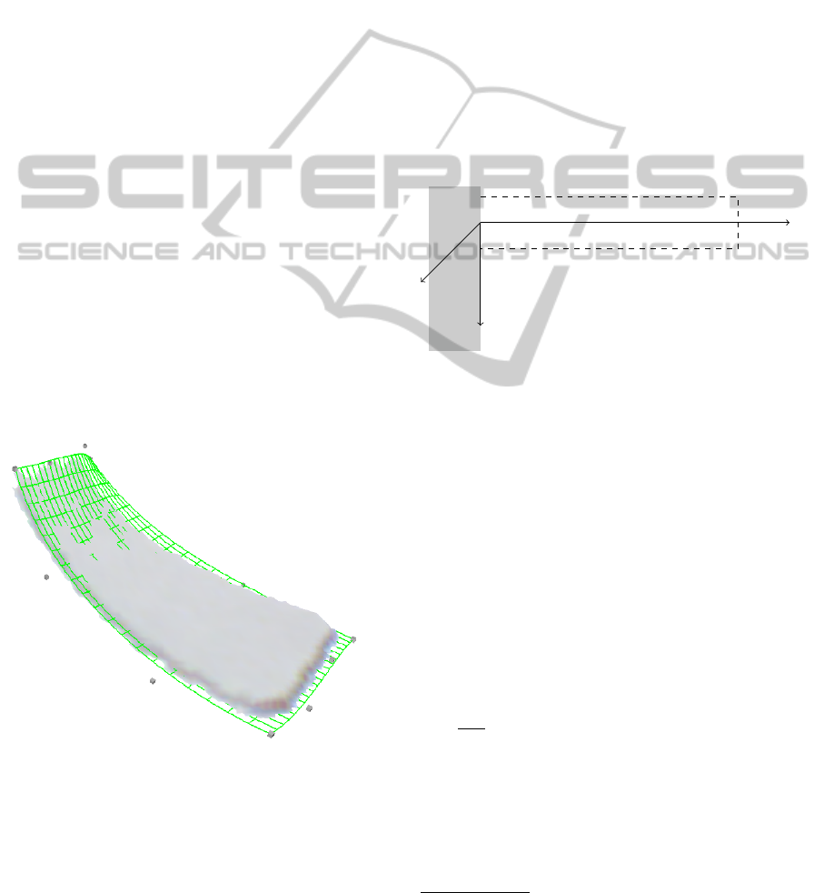
As demonstrated by (Jordt et al., 2011) a real-

time tracking of a detailed 3D mesh, using depth and

colour video from a Kinect camera, can be coupled to

a low-dimensional NURBS surface, see Figure 2.

Figure 2: A scanned 3D mesh of an object and its associ-

ated NURBS surface (Figure courtesy of (Jordt et al., 2011),

with kind permission by the authors).

Similarly we decouple the geometry from the de-

formation. Only the deformation of the control points

in the NURBS surface is used as a a parameter in the

learning stage.

The deformation modelling is thus reduced to the

problem of ﬁnding the deformation for the control

points of the NURBS surface. When at some point

the whole surface deformed geometry is needed (for

instance for collision detection), it is derived from the

deformed control points. Having a deformation that

models to the NURBS surface also enables easier cou-

pling to the NURBS based deformation tracking.

3.1.2 Choice of Model

The Bernoulli-Euler (BE) beam theory has since its

development in the 18th century, been a core element

in structural engineering. Its’ formulation and param-

eters are readily understandable, and many problems

have analytical solutions. It is a simple model how-

ever, as it only accounts for the bending moment and

lateral displacement of the beam.

ﬁxed end

free end

Figure 3: A cantilevered beam.

Several additional models have been developed

during the years to improve on the BE model. Most

noteworthy of these is the Timoshenko model (Timo-

shenko, 1921), which takes into the account both ro-

tation inertia and shear deformation.

To account for the additional effects, the Timo-

shenko model adds a dependent variable to account

for the angular displacement and a parameter known

as the shape factor. The shape factor is a function of

Poisson’s ratio for the material, the wave frequency

and the shape of the cross section. For the static case,

the shape of the cross section is the most dominant

effect on the shape factor

The slenderness ratio is the ratio of the beam

length to the radius of gyration, calculated as

I/A. It characterizes the magnitude of differ-

ent forces involved in the beam equations. In the

work of (Seon M. Han, 1999) they recommend the

use of the simple BE model for large slenderness ra-

tios (s > 100), and the Timoshenko model for smaller

ratios where second order effects of rotation and shear

become important.

Poisson’s ratio varies for normal materials only be-

tween 0 and 0.5 (Landau et al., 1986).

ICAART 2012 - International Conference on Agents and Artificial Intelligence

626

For our present experiments, we target moderately

slender objects (100 < s < 150). Accordingly we use

the BE beam theory.

3.1.3 Bernoulli-Euler Beam Theory

The governing equation for the dynamic BE beam can

be formulated as a partial differential equation in the

deﬂection w of the beam

∂

∂x



∂

∂x



= −µ

∂

∂t

+ q (2)

where w(x,t) is the deﬂection as a function of position

x on the beam and time t. E is Young’s modulus, I is

the second moment of inertia and q the is body load.

Young’s modulus, E is a material dependent pa-

rameter and represents the stiffness of the material.

It may be either measured or derived from tabulated

data. For homogeneous materials it is a constant.

The second moment of inertia, I is a geometry de-

pendent parameter, quantifying resistance to bending

at a given cross section. It is deﬁned as I =

dA,

where z is the height of the cross section, being per-

pendicular to the bending. For a geometry that has a

constant cross section (e.g. a simple beam) it is a con-

stant. For the special case of a rectangular cross sec-

tion with height h and width b, I is equal to bh

/12.

This suggests a strong dependence of the thickness of

such a beam, to the resulting deformation, i.e. varying

the thickness will give the strongest resulting change.

The body load, q represents an external force act-

ing upon the beam. It is deﬁned as a force per unit

length. Point forces may be modelled with the use of

the Dirac delta function.

For the static case of a homogeneous beam with

constant cross section, Equation 2 reduces to the or-

dinary differential equation (ODE)

= q(x) (3)

where w(x) is the deﬂection now only as a function of

position, and E and I are both constants.

The static beam equation, Equation 3 is a fourth-

order ODE. In order to ﬁnd a unique solution for

the deformation proﬁle w(x), four boundary condi-

tions must be prescribed. Assuming that the gripper

is placed such that the left end of the object at x = 0 is

ﬁxed in space (both deﬂection and slope equal to zero)

we have the boundary conditions for the clamped end

x=0

= 0 ;

∂w

∂x



x=0

= 0 (4)

For the other end of the object at x = L, we pre-

scribe the boundary conditions (both the bending mo-

ment and the shear force in the beam is zero) corre-

sponding to that this part of the object is free to move

∂

∂x



x=L

= 0 ;

∂

∂x



x=L

= 0 (5)

The ODE Equation 3 together with the boundary

conditions Equation 4 and Equation 5 form a bound-

ary value problem. The solution gives the deﬂection

of a ﬁxed-free/cantilevered beam, as depicted on Fig-

ure 3.

This boundary value problem, along with the re-

striction that the load is uniformly distributed i.e.

q(x) = constant, has the analytical solution to the de-

ﬂection w(x) of the beam

w(x) =

(6L

− 4Lx + x

)

24EI

(6)

3.2 Object Description

One aim of the action learning is to be able to apply

an action learned with one object to another object

that behaves similarly. The behaviour of an object is

considered to be deﬁned by the deformation that oc-

curs when a speciﬁc grasp is applied and the object is

affected by gravity - these deformations can be mod-

elled as outlined in section 3.1.

In the following the condensation of the high-

dimensional information that is intrinsic to the defor-

mation modelling into a feature vector of lower di-

mensionality is described. Ideally two different ob-

jects, e.g. with different shapes, maps to the same

feature vector if they behave identically, such that the

same action can be applied.

In order to achieve a feature-vector that is compa-

rable across objects, the NURBS surfaces describing

the undeformed object S

(u,v) and the object in a hor-

izontal orientation, affected by gravity S

(u,v). The

length of the objects is normalized.

The difference between the two surfaces describes

how much the object has deformed at the individual

locations:

S(u,v) = S

(u,v) −S

(u,v) (7)

Based on a regular grid g of size I × J, the defor-

mations are obtained at a set of discrete locations and

for a feature vector f :

f =



S (g

)k,...,k

S(g

i j

)k,....,k

S(g



(8)

where g

i j

refers to the a point of the grid at the posi-

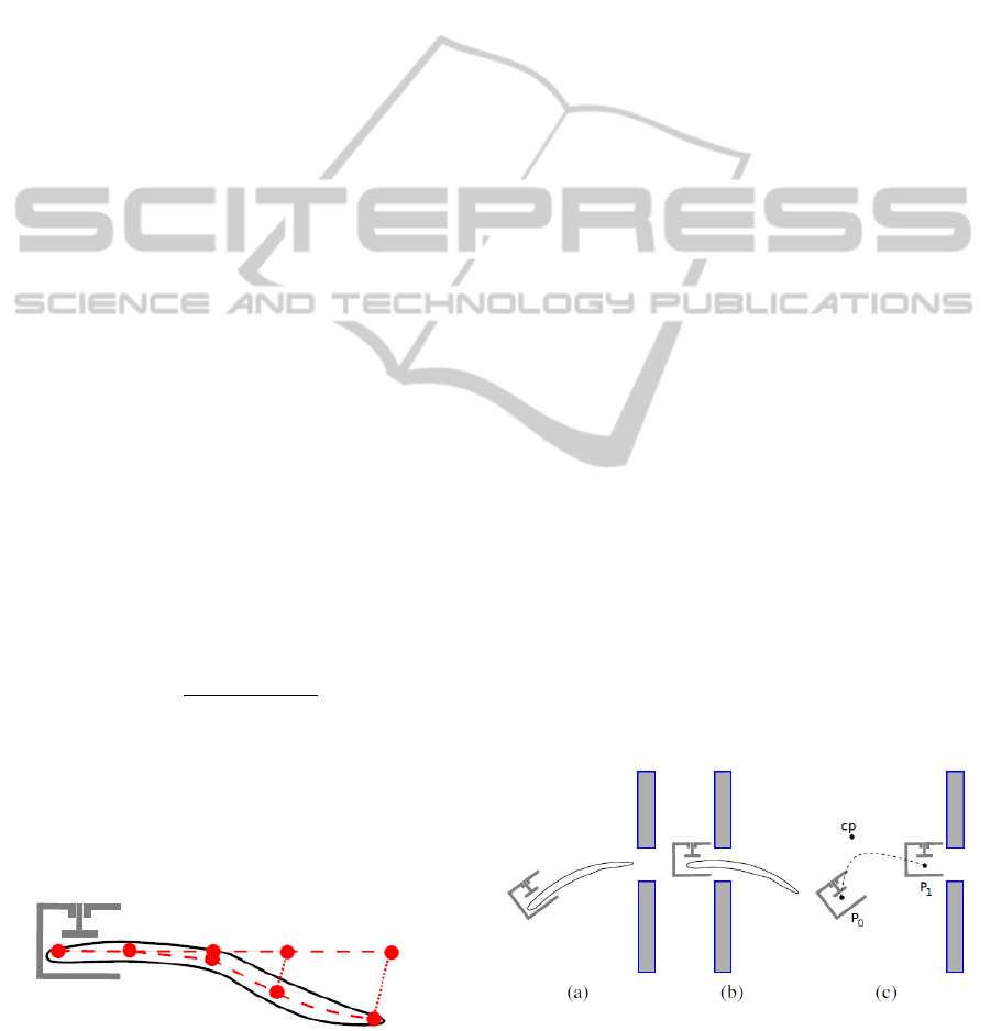
tion (i, j). An simpliﬁed example for the calculation

of f is shown in Figure 4. It correspond to a deﬂect-

ing beam where the deﬂections can be described by a

NURBS curve instead of an entire surface.

LEARNING PEG-IN-HOLE ACTIONS WITH FLEXIBLE OBJECTS

627

3.3 Action Learning

The exact 6D trajectory of a Peg-In-Hole operation

depends both on the elastic behaviour of the object,

the grasp applied to the object and the shape of the

object. However, although the 6D trajectory for in-

stance varies with the size of the object, it might still

share similarities with other Peg-In-Hole actions. The

parametrization of the action aims to reduce the com-

plexity of the learning problem and eases the transfer

of a learned action from one object to another as the

object does not need to be identical, but only to share

certain properties. The following sections cover the

parametrization of Peg-In-Hole actions as well as the

structure and strategy for learning them.

3.3.1 Action Parametrization

The Peg-In-Hole action is deﬁned by a trajectory

which the robot executes. The endpoint P

is known

as it is directly in front of the hole. The startpoint P

is obtained online utilizing the deformation prediction

and ensures that the end of the object is horizontal and

in front of the hole (see Figure 5). The trajectory from

the start to the endpoint is considered to be approxi-

mated by a curve deﬁned by two-dimensional trans-

lations and one-dimensional rotations. The points P

and P

are therefore both points in R

× SO(2).

The curve P(t) is deﬁned using a rational B

ezier-

curve (Piegl and Tiller, 1997) based on three control

points: the start and endpoint as well as one additional

controlpoint which will be obtained by learning:

P(t) = P

+ B(t)(P

− P

) for t ∈ [0; 1] (9)

with

B(t) =

∑

i=0

i,n

(t)P

∑

i=0

i,n

(t)w

(10)

where b

i,n

(t) is the Bernstein polynomial with n = 2

and P

refers to the i’th controlpoint for the curve:

∈ {0, cp,1} (11)

Figure 4: Illustration of the differences between the unde-

formed mesh (straight dashed line) and the deformed mesh

(bent dashed line) used for the feature vector in a 2D case.

The resulting feature vector will be 5-dimensional.

The weights are ﬁxed, w = [1,2,1], which ensures

that the second control point, cp, has an increased im-

pact. Thereby also motions that lead to a signiﬁcant

overshoot can be learned.

Note that the control points do not depend on the

scale of the motion or the object (see Equation 9).

Therefore a learned control point will lead to mean-

ingful trajectories for any object, although it is not

guaranteed that the performed action will be success-

ful.

3.3.2 Action Learning Framework

The set of potentially successful Peg-In-Hole actions

is modelled using Kernel Density Estimation (Silver-

man, 1986). Every time a control point that leads to a

successful action has been obtained, it is added to the

density d. However, contrary to the situation in (De-

try et al., 2011) where grasp affordances are learned

for a speciﬁc object, we cannot assume the objects to

be identical. Therefore a kernel, K

µ,σ

(cp, f ), which is

a compound of two kernels is used: one reﬂecting the

Peg-In-Hole action as such, the other reﬂecting the

object features speciﬁed in section 3.2.

µ,σ

(cp, f ) = N

PiH

,σ

(cp)N

Ob ject

,σ

( f ) (12)

where N

PiH

and N

Ob ject

are isotropic multivariate

Gaussian kernels located at the mean positions µ

resp. µ

and with bandwidth of σ

resp. σ

. The

density is given by a weighted sum of the m kernels:

d(cp, f ) =

∑

i=0

,σ

(cp, f ) (13)

where the weights w

ensure that the density integrates

to one, hence

∑

= 1.

During the learning every controlpoint that leads

to a successful action will contribute to the density

Figure 5: Illustration of (a) starting conﬁguration P

and

(b) target conﬁguration P

for the Peg-In-Hole action. (c)

shows a projection of the 3D trajectory based on P

, P

and

the controlpoint cp.

ICAART 2012 - International Conference on Agents and Artificial Intelligence

628

with one particle. Assuming that an action is either

successful or not, all particles of the density have

equal weights. Given an uniformly sampled search

space, the value of the density at a given point will

be proportional to the likelihood of the corresponding

action for being successful.

Here, we choose the points for the feature vector

f as those illustrated in Figure 4. It should be no-

ticed that the point P

is scaled with respect to object

length (see Figure 4). Thus, two objects with differ-

ent lengths having the same feature vector then have

equivalent shapes and may be handled in the same

way except for choosing the appropriate length scaled

. Thus, the parameters cp and f covers a given con-

trol point and shape for all object lengths.

Assume now that we wish to solve a Peg In Hole

action for a hitherto unstudied object. The deﬂection

model is then used to compute the feature vector f

Then the control point with the highest probability for

success can be obtained by searching for the maxi-

mum of the density d(cp, f

3.3.3 Action Learning Strategy

The system is not provided with any prior knowledge

to bootstrap the learning strategy. Therefore a 2-step

learning mechanism has been considered. First, an

exhaustive search on the controlpoints is performed

in a simulated environment. As the controlpoints are

3-dimensional it is feasible to explore the space with

a reasonable resolution. The outcome of the sim-

ulated experiments leads to a density as deﬁned in

Equation 13. Examples for the clouds of particles are

shown in Figure 7. Finally, the density achieved by

simulation can be sampled and evaluated on the real-

world setup, leading to a new density.

Utilizing a simulator does not only allow the eval-

uation of large set of experiments, it also provides a

detailed feedback about the performed action. The

outcome of an experiment is therefore not only a bi-

nary, namely success or failure, but also the minimal

clearance c between the object and rim of the hole that

is experienced during the individual experiment. A

bigger clearance implies that the action is more robust

to external disturbances and modelling errors. This

fact is reﬂected by the weights:

i j

∑

j=0

i j

(14)

where c

i j

is the minimal clearance of the j’th out of M

successful experiments with the i’th object, given N

objects in total. Thereby the maximum of the density

does not only reﬂect the success likelihood, based on

the statistics of the samples, but directly corresponds

Figure 6: Approximation of a ﬂexible object using a rigid

device. Self-collisions within the simpliﬁed object model

are ignored.

to the action that is expected to be the most robust in

the given situation.

4 EXPERIMENTS

In the following the simulated experiments used to

bootstrap the learning are described in section 4.1.

Experiments on the real setup are described in section

4.2.

The test specimens are cuboid pieces of silicone

rubber, cut from a sheet of 2.0 mm thickness, into

pieces of 15 mm width. The density of the silicone

sheet as given by the manufacturer is 1.15 g/cm

and

the shore A hardness is 60 ± 5 (which corresponds to

a Young’s modulus of approximately 3.6 MPa).

4.1 Simulated Experiments

For the simulation, based on a simulation environ-

ment from (Ellekilde and Jørgensen, 2010), a ﬂexi-

ble, cuboid object is approximated by a rigid device

consisting of a set of consecutive boxes as illustrated

in Figure 6. This approximation allows for efﬁcient

collision detections as well as clearance calculations

- the precision can be controlled easily by adjusting

the number of joints in the device. The angles of the

joints connecting the boxes are obtained from the ob-

ject deformation modelling which takes the orienta-

tion of the grasped object with respect to gravity into

account.

Table 1: Overview over the different outcomes experienced

in the simulator.

Minimal clearance [mm]

Object collision 0 - 2 2 - 4 4 <

80 mm long 6899 258 288 555

60 mm long 4711 416 524 2349

40 mm long 3418 678 1267 2637

LEARNING PEG-IN-HOLE ACTIONS WITH FLEXIBLE OBJECTS

629

Simulations have been done for three different ob-

jects, testing Peg-In-Hole actions for each object with

8000 controlpoints. The outcomes of the experiments

(summarized in Table 1) indicate that it is easier to

insert short objects rather than long ones: a higher

proportion of all actions succeeded and the average

minimal clearance of the succeeding actions is larger.

This has been expected as long objects lead to large

deﬂections and can thus not be inserted by a close to

straight-line motion in contrast to short objects.

All controlpoints learned for the short resp. long

object are shown in Figure 7. In both cases the so-

lutions form a close to convex area which indicates

that the complete density can be approximated with a

sparse density consisting of fewer particles, but with

larger bandwidths. As the costs of the search for a

maximum within the density depend on the number

particles that need to be evaluated, densities based on

fewer particles ease the implementation of a real-time

system.

Figure 7: Illustration of the 3D point clouds of the control-

points that lead to successful actions for the (a) 40 mm long

object and (b) the 80 mm long object.

4.2 Real Experiments

In the following the validity of the modelled deﬂec-

tions as well as the learned Peg-In-Hole actions are

assessed by real-world experiments.

4.2.1 Deformation Validation

To validate the modelling, the maximum deformation

of each test object have been measured in a separate

experimental setup.

For the test objects of 80,60 and 40 mm, the mean

values for the deformations are respectively 29.25,

10.25 and 2.25 mm. Using the tabulated shore A

hardness of 60 for the silicone rubber (correspond-

ing Young’s modulus 3.6 MPa), the deformation is

overestimated. This trend is clear for the larger de-

formations of the piece 80 mm in length. Using an

extrema of the hardness, shore A 65 (Young’s mod-

ulus 4.4 MPa) the maximum calculated deﬂection of

Table 2: The maximum deﬂection of the respective test

objects. The last column shows the deformation as calcu-

lated by the modelling, assuming a shore A hardness of 60.

For each object, 4 different orientations have been indepen-

dently measured.

Measured max. deﬂection [mm]

Object

O1 O2 O3 O4

Sim.

80 mm

29 28 30 30

33.5

60 mm

10 10 10 11

10.5

40 mm

2 2 3 2

2.5

the piece reduces to 28.3 mm, which is closer to the

observed mean of 29.25 mm.

4.2.2 Peg-in-Hole Actions

Based on the results of the simulated experiments,

Peg-In-Hole actions with the simulated objects have

been evaluated on the real setup. The controlpoints

have been obtained by searching the density obtained

by simulation for a maximum. The resulting actions

have been observed to be successful, the last step of

the insertion of the longest object is shown on Fig-

ure 1. However manual measurements of the mini-

mal clearance have been done in order to investigate

the robustness of the learned actions. Especially for

the longest object, the clearance has been observed to

be approximately 1 mm (for the 80 mm long object)

which is lower than expected according to results in

Table 1.

A potential reason for smaller clearance might be

caused by alignment errors between the grasped ob-

ject and the hole as even small errors seam to have a

signiﬁcant effect. Further the most signiﬁcant differ-

ence between measured and expected clearance has

occurred for the 80 mm long object, which might be

correlated with the fact that the deﬂection modelling

for this object had the bigger error than the others (see

Table 2).

5 FUTURE WORK

The overall system discussed so far is, as no sen-

sor input is used to correct for modelling errors, an

open-loop system. However, when the complete sce-

nario is considered where an object becomes scanned,

modelled, grasped and inserted multiple error sources

arise. If the object-relative location of the grasp is sig-

niﬁcantly different than expected, this would have an

impact on the modelling and might cause the Peg-In-

Hole action to fail.

ICAART 2012 - International Conference on Agents and Artificial Intelligence

630

To counteract potential errors an additional Kinect-

camera is introduced, enabling the system to super-

vise the Peg-In-Hole operation. We foresee that the

additional feedback can be used to:

• Improve the deﬂection modelling over time.

• Correct for inaccuracies during the grasping.

• Correct the starting position of the Peg-In-Hole

action.

6 DISCUSSION

In this paper we presented a system to perform Peg-

In-Hole action with ﬂexible objects. The system uti-

lizes a physical modelling of the elastic behaviour of

the objects and an action learning mechanism based

on kernel density estimation. Objects are identiﬁed by

a distinctive feature vector that enables the system to

recognize objects with similar behaviours as known

objects. Thereby previously learned actions can be

applied to new objects, with similarly behaviour as

known ones. This enables the system to perform in

real time as the demand for time consuming mod-

elling operations is minimized.

ACKNOWLEDGEMENTS

This work was co-ﬁnanced by the INTERREG 4 pro-

gram Syddanmark-Schleswig-K.E.R.N. by EU funds

from the European Regional Development Fund. The

presented work has also received funding from the EU

Seventh Framework Programme under grant agree-

ment no. 270273, Xperience.

REFERENCES

Anshelevich, E., Owens, S., Lamiraux, F., and Kavraki,

L. E. (2000). Deformable volumes in path planning

applications. In IEEE International Conference on

Robotics and Automation.

Bardinet, E., Cohen, L. D., and Ayache, N. (1995). A para-

metric deformable model to ﬁt unstructured 3d data.

Bruyninckx, H., Dutr

e, S., and Schutter, J. D. (1995). Peg-

on-hole: A model based solution to peg and hole

alignment. In International Conference on Robotics

and Automation.

Detry, R., Kraft, D., Kroemer, O., Bodenhagen, L., Peters,

J., Kr

uger, N., and Piater, J. (2011). Learning grasp

affordance densities. Paladyn Journal of Behavioral

Robotics, 2:1–17.

Ellekilde, L.-P. and Jørgensen, J. A. (2010). RobWork: A

Flexible Toolbox for Robotics Research and Educa-

tion. In International Symposium on Robotics,

Jim

enez, P. (2011). Survey on model-based manipula-

tion planning of deformable objects. Robotics and

Computer-Integrated Manufacturing, In Press.

Jordt, A., Fugl, A. R., Bodenhagen, L., Willatzen, M.,

Koch, R., Petersen, H. G., Andersen, K. A., Olsen,

M. M., and Kr

uger, N. (2011). An outline for an in-

telligent system performing peg-in-hole actions with

ﬂexible objects. In The International Conference on

Intelligent Robotics and Applications (Accepted).

Landau, L. D., Pitaevskii, L. P., Lifshitz, E. M., and Kose-

vich, A. M. (1986). Theory of Elasticity. Butterworth-

Heinemann.

Meitinger, T. and Pfeiffer, F. (1996). The spatial peg-in-

hole problem. In Proceedings of the Second World

Automation Congress, Montpellier, France.

Piegl, L. and Tiller, W. (1997). The NURBS book. Springer-

Verlag New York, Inc., New York, NY, USA, 2. edi-

tion.

Samareh, J. A., Samareh, J. A., and Polynomial, B. B.

(1999). A survey of shape parameterization tech-

niques.

Seon M. Han, Heym Benaroya, T. W. (1999). Dynamics of

transversely vibrating beams using four engineering

theories. Journal of Sound and Vibration, 225:935–

988.

Silverman, B. W. (1986). Density Estimation for Statistics

and Data Analysis. Chapman and Hall/CRC.

Timoshenko, S. P. (1921). On the correction for shear of

the differential equation for transverse vibrations of

prismatic bars. Philosophical Magazine, 41:744–746.

Villarreal, A. and Asada, H. (1991). A geometric rep-

resentation of distributed compliance for the assem-

bly of ﬂexible parts. In International Conference on

Robotics and Automation.

Xia, Y., Yin, Y., and Chen, Z. (2006). Dynamic analysis for

peg-in-hole assembly with contact deformation. In-

ternational Journal of Advanced Manufacturing Tech-

nologies, 30:118–128.

LEARNING PEG-IN-HOLE ACTIONS WITH FLEXIBLE OBJECTS

631