PARALLEL R-CENTIPEDES

Fast Contour Extraction for 3D Visualization

Mehdi Nouri Shirazi and Yoshiyuki Kamakura

Faculty of Information Science and Technology, Osaka Institute of Technology, Osaka, Japan

Keywords:

Deformable Contours, Active Contours, Electron-microscope Tomographic Images, 3D-visualization.

Abstract:

In our previous article, we introduced a class of region-based deformable contour models called R-centipedes.

The R-centipedes are able to operate in three modes: 1) deﬂationary, 2) inﬂationary, or 3) a mixture of both.

We demonstrated that the deﬂationary R-centipedes could adaptively change their structures in order to ex-

tract structures of interest and their substructures from complex Electron Microscope (EM) tomography slice

images. The R-centipedes have several desirable features such as 1) structural ﬂexibility which allows them

to extract multiple objects in a single slice image, 2) high accuracy, and 3) insensitivity with respect to their

initial positions and conﬁgurations. In this article, we introduce two parallel versions of the R-centipedes, 1)

implicit, and 2) explicit parallel R-centipedes. We present three simulation studies to demonstrate their ﬂexi-

bility, effectiveness and computational efﬁciency in extracting structures in three different complex situations.

1 INTRODUCTION

Extracting meaningful structures of interest and their

internal structures from medical and EM tomographic

slice images for 3D visualization is a challenging

problem. This is due to the complexity and variabil-

ity of the biological structures that are usually em-

bedded in intensity inhomogeneities, imaging noise,

textural artifacts and boundary irregularities, the large

size (> 1000 × 1000 pixels) and numerous number

(> 256 slices) of tomographic images that should be

processed. The challenge is to extract the bound-

ary pixels belonging to the structures of interest from

each slice image and integrate them into complete and

consistent 3D representations of the objects and their

parts as fast as possible and preferably with no or min-

imal user interaction.

Deformable contour models (McInerney and Ter-

zopoulos, 1996), including the standard energy-

minimizing snakes (Kass et al., 1988) and balloons

(Cohen, 1991), offer an attractive approach to con-

tour extraction problem and have been used broadly

in image segmentation. The active contours move and

deform within the slice images under a combined in-

ﬂuence of internal and external forces.

Though the standard deformable models have

proved to be very useful tools in 3D visualization they

suffer from some characteristic limitations. First, they

should manually be initialized close to the boundaries

of the target objects. Second, the segmentation results

might be dependent on the positions of the initial con-

tours. Third, they are geometrically inﬂexible due to

inability to re-parametrize. Finally, they are incapable

of adapting to object topology.

To overcome the limitations of the standard

snakes, McInerney and Terzopoulos (McInerney and

Terzopoulos, 1995) augmented the snakes with re-

parametrization, splitting and merging mechanisms

using the afﬁne cell image decomposition (ACID)

technique. They showed that their topology adaptive

snakes, called the T-snakes, could successfully extract

multiple objects and even grew into structures with

complex geometries in different medical image anal-

ysis scenarios.

Almost all the standard explicit snakes and their

topology adaptive versions are edge-based models.

There are several well known problems with edge-

based snakes. First, edge-based snakes use edge de-

tector to stop their evolving contours on the bound-

aries of the target objects. Second, if the image is

noisy, the image should be smoothed isotropically. If

the image is very noisy, the Gaussian smoothing has

to be strong which will smooth the stopping edges

too. Third, to get rid of spurious weak edges the

user has to set a threshold, which is usually a criti-

cal parameter that directly affects the quality of the

segmentation result. Fourth, the edge-based models

are inapplicable in cases where the boundaries of the

713

Nouri Shirazi M. and Kamakura Y..

PARALLEL R-CENTIPEDES - Fast Contour Extraction for 3D Visualization.

DOI: 10.5220/0003825807130718

In Proceedings of the International Conference on Computer Graphics Theory and Applications (IVAPP-2012), pages 713-718

ISBN: 978-989-8565-02-0

 2012 SCITEPRESS (Science and Technology Publications, Lda.)

Figure 1: The neighboring nodes of a closed centipede are

coupled through the elasticity and rigidity parameters, ω

target objects are not necessarily deﬁned by gradients.

Fifth, they easily get stuck with textural artifacts.

These limitations seriously mitigate the applica-

bility of the edge-based snakes in complex situations

in general, and in EM tomography image analysis

and 3D visualization in particular, where demands are

high for speed, accuracy and automation with no or

minimal user interaction.

In our previous article (Shirazi and Kamakura,

2010), we introduced a class of region-based topo-

logically ﬂexible deformable models that we called

restructuring centipedes (R-centipedes). In this ar-

ticle, we introduce two parallel versions of the R-

centipedes dubbed explicit parallel R-centipedes and

implicit parallel R-centipedes. Our experiments with

the parallel R-centipedes have shown that they are

structurally ﬂexible enough: 1) to extract structures

with complex boundaries from EM tomography slice

images when operating in their deﬂationary mode,

and 2) grow into micro-tubular complex structures

with high speed and accuracy when operating in their

inﬂationary mode.

2 RESTRUCTURING

CENTIPEDES

A closed centipede consists of a number of self-

powered two-legged moving automatons (nodes),

where the neighboring nodes are coupled as shown in

Fig. 1. The legs are facilitated with sensory patches

whereby the centipedes can interact with their envi-

ronments.

Restructuring centipedes (R-Centipedes) are de-

formable centipedes which can restructure themselves

by, 1) recruiting new nodes, 2) removing nodes, 3)

splitting into new R-centipedes, and 4) merging with

the other R-centipedes that they might come into con-

tact.

As shown in Fig. 2, with each node there are asso-

ciated, 1) one inner patch P

i,k

, 2) one outer patch P

o,k

and 3) a self-powered moving force

While R-centipedes undergo deformation and re-

structuring, their nodes are assumed to keep the axes

of their inner and outer patches aligned and perpen-

Figure 2: The inner patch P

i,k

, outer patch P

o,k

, self-

powered moving force

, and the external force

at node

dicular to the lines passing through their two neigh-

boring nodes, as shown in Fig. 2.

2.1 Deformation Equations

Let~v

(t) = [x

(t) y

(t)]

denote the time-varying po-

sition vector of node k. The dynamical behavior of a

closed deformable centipede that consists of N cou-

pled self-powered moving nodes is assumed to be

governed by the following motion equations

−

, (1)

for all k = 0,...,N − 1. The ﬁrst term of Eq. (1),

denotes the velocity of node k,

and

are image-

independent internal forces known as the tensile force

and the ﬂexural force at node k, respectively,

is a

self-powered moving force at node k, and ﬁnally

an external force which the image might exert at node

The internal tensile and ﬂexural forces are given

(t) = ω

∆

(t), (2)

and

(t) = ω

∆

(∆

(t)), (3)

respectively, where the 2nd-order difference operator

∆

is given by

∆

(t) = (~v

k−1

(t) − 2~v

(t) +~v

k+1

(t))/(∆l(t))

. (4)

In the above equations, the parameter ω

controls

the resistance of the centipede to expanding and/or

shrinking, whereas ω

controls the resistance of the

centipede to bending at its nodes, and ﬁnally ∆l(t)

denotes the time-varying distance between the imme-

diate neighboring nodes. For closed centipedes, all

indexes in the above expressions is interpreted mod-

ulo N.

The self-powered moving forces are given by

(t) = c

(t), (5)

IVAPP 2012 - International Conference on Information Visualization Theory and Applications

714

where ~n

(t) denotes a time varying vector deﬁned as

a unit vector perpendicular to the line passing through

the k-th node’s immediate two neighboring nodes.

The constant c

controls the magnitude of the self-

powered forces. When all nodal self-powered forces

are exerted inwardly the R-centipede shrinks (deﬂa-

tionary R-centiped), when all exerted outwardly it ex-

pands (inﬂationary R-centiped), and when partly in-

wardly and partly outwardly we will have deﬂation-

ary/inﬂationary R-centipedes which can be used in

object tracking problems.

The last components which affect the behaviors

of R-centipede are the time-varying external forces

(t). The concrete form of these forces are in gen-

eral application dependent. Here, we deﬁne them

as image-dependent stopping forces which can even-

tually bring the deformation process to halt at the

boundaries of the objects of interest.

Let P

i,k

(t), and P

o,k

(t) denote the sets of the lo-

cations of the pixels that come under the inner and

outer patches of node k at time t, respectively. Let

i,k

(t) and m

o,k

(t) denote the mean values of the gray-

levels of the pixels belong to P

i,k

(t), and P

o,k

(t), re-

spectively, by

i,k

(t) =

| P

i,k

(t) |

∑

(i, j)∈P

i,k

(t)

I(i, j), (6)

o,k

(t) =

| P

o,k

(t) |

∑

(i, j)∈P

o,k

(t)

I(i, j), (7)

where | P

i,k

(t) |, and | P

o,k

(t) | are the cardinal num-

bers of P

i,k

(t) and P

o,k

(t), respectively.

Furthermore, let

(t) and m

(t) denote the means

of m

i,k

(t) and m

o,k

(t) and σ

(t) their stan-

dard deviations. Then, the external nodal forces for

the deﬂationary R-centipedes are deﬁned by

(t) =



−

(t), if m

i,k

(t) ≥

) + c

)

0, otherwise,

(8)

and for the infalationary R-centipedes by

(t) =



−

(t), if m

o,k

(t) ≤

) + c

)

0, otherwise.

(9)

Here the constant c

controls the degree of textural

mismatching that is tolerated, and t

denotes the time

when the R-centipede is created and set free to move

and deform.

2.2 Restructuring Rules

The R-centipedes are allowed to restructure by, 1) re-

cruiting (adding) new nodes, 2) dismissing (deleting)

nodes, and 3) splitting. They add and delete nodes in

order to keep the lengths of their two-node segments

approximately constant. They check the lengths of

their segments after each incremental deformation,

add a new node in the middle of any segment which

they ﬁnd to be too long, and/or delete one of the two

nodes of any segment which they ﬁnd to be too short.

Active R-centipedes are also allowed to split into two

R-centipedes whenever they detect a self-crossing.

The ability to split enable the R-centipedes, ﬁrstly,

to generate the same ﬁnal conﬁgurations regardless of

their initial positions/conﬁgurations taht encompass

the objects of interest, secondly, to extract multiple

objects in slice images, and thirdly, not get stuck with

textural artifacts which exist rampantly in EM tomog-

raphy slice images.

2.3 Non-parallel Incremental

Deformation Rule

To solve the motion equations of a deﬂationary R-

centipede deﬁned by Eqs. (1)-(6) and (8), or an inﬂa-

tionary R-centipede deﬁned by Eqs. (1)-(7) and (9),

we used the implicit Euler method in our previous

article (Shirazi and Kamakura, 2010). The implicit

Euler method approximates the temporal derivatives

with forward ﬁnite differences. It updates the x- and

y-components of the positions of nodes from time t to

time t + ∆t according to the following 2N system of

nonlinear equations

(I + ∆tC(t))

V(t + ∆t) =

V(t) + ∆t(

F(t) +

Γ(t)), (10)

where I denotes the (N(t) × N(t))-dimensional iden-

tity matrix, whereas C(t) denotes an (N(t) × N(t))-

dimensional matrix known as the stiffness matrix (for

detail, see (Shirazi and Kamakura, 2010)).

In the above equation,

V(t) =

[~v

(t)...~v

N(t)−1

(t)]

denotes the N(t)-dimensional

vectors of the locations of the centipede’s nodes at

time t, whereas

Γ(t) = [

(t)...

N(t)−1

(t)]

denotes

the N(t)-dimensional vectors of the self-powered

moving nodal forces, and

F(t) = [

(t)...

N(t)−1

(t)]

denotes the the image-dependent stopping forces at

time t.

3 PARALLEL INCREMENTAL

DEFORMATION RULES

By expanding Eq. (1) at the node k, and by using Eqs.

(2)-(4) we will get

− c

k−2

− c

k−1

− c

k+1

− c

k+2

. (11)

PARALLEL R-CENTIPEDES - Fast Contour Extraction for 3D Visualization

715

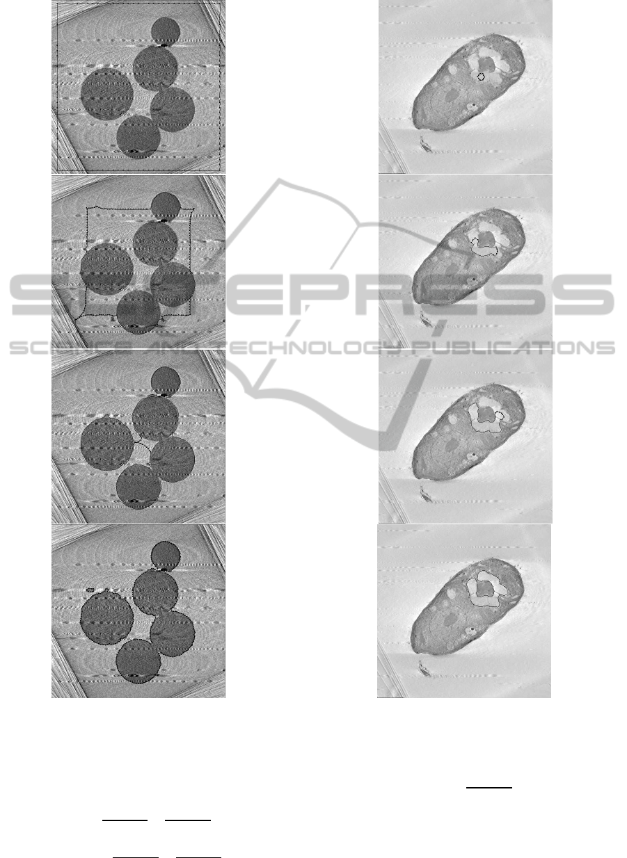
Figure 3: Deﬂationary mode: snap shots of the contour ex-

traction process. The bottom image shows the ﬁnal posi-

tions/conﬁgurations of the four R-centipedes that generated

and survived in the process.

where c

, c

and c

are given as

2ω

(∆l(t))

6ω

(∆l(t))

, (12)

= −

(∆l(t))

−

4ω

(∆l(t))

, (13)

Figure 4: Inﬂationary mode: snap shots of the contour ex-

traction process. The bottom image shows the extracted

boundary of a clicked substructure of an alga.

(∆l(t))

. (14)

By using the implicit Euler method we can dis-

cretize Eq. (11) in time domain and get

IVAPP 2012 - International Conference on Information Visualization Theory and Applications

716

Figure 5: Inﬂationary mode: snap shots of the extraction

process. The bottom image shows the extracted boundary

of a micro-tubular structure.

(1+∆tc

)~v

(t + ∆t) = ~v

(t)

− (c

k−2

(t) + c

k−1

(t)

+ c

k+1

(t) + c

k+2

(t))∆t

+ (

(t) +

(t))∆t, (15)

and by using the explicit Euler method we get

(t + ∆t) = (1− ∆tc

)~v

(t)

− (c

k−2

(t) + c

k−1

(t)

+ c

k+1

(t) − c

k+2

(t))∆t

+ (

(t) +

(t))∆t. (16)

The rules given by the updating Eqs. (15) and (16)

are two different parallel versions of the non-parallel

incremental deformation rule given by the updating

rule (10).

4 SIMULATION EXPERIMENTS

4.1 Experiment 1

We applied the deﬂationary non-parallel and the two

parallel R-centipedes to the 500× 500 test EM slice

image shown in Fig. 3. We initiated 4-node R-

centipedes and positioned them near the frame of the

test image and let them move, deform, split and adapt

their nodes until they stabilized and stopped. The

upper three images show the snap shots of the in-

termediate positions and conﬁgurations of the deﬂa-

tionary implicit parallel R-centipede at three differ-

ent instances. Though the intermediate positions and

conﬁgurations of the non-parallel and explicit paral-

lel R-centipedes were different, their ﬁnal conﬁgura-

tions were almost the same to such extend that we

decided not to put them here for the sake of space.

We used the same parameters for the non-parallel

and parallel R-centipedes. The parameters used in

the simulation were: ω

= 0.2, ω

= 0.4, γ

= 300,

= 2.5, H

= H

= 4 (pixels), W

= W

= 7 (pixels),

∆l(t) = ∆l = 5 (pixels), and ∆t = 0.01.

This experiment clearly shows that, regardless

of the numerous textural artifacts scattered over the

background, the parallel R-centipedes like their non-

parallel predecessor are able to extract the contours of

the objects of interest with high precision.

The cpu-time that the non-parallel R-centipede

used was 6.18 seconds, while the two parallel R-

centipedes used about 1.93 seconds each.

4.2 Experiment 2

In our second experiment designed to demonstrate the

effectiveness and the speed of the proposed inﬂation-

ary parallel R-centipedes, we applied the non-parallel

and parallel R-centipedes to the 512 × 512 EM slice

image of an alga shown in Fig. 4.

The R-centipedes were initiated by a mouse click

on the internal substructure of interest and were let

PARALLEL R-CENTIPEDES - Fast Contour Extraction for 3D Visualization

717

free to move, deform, split and adapt their nodes until

they stabilized and stopped.

The three upper images of Fig. 4 show the inter-

mediate positions/conﬁgurations of the implicit par-

allel R-centipede at different instances, whereas the

bottom image shows the result of the contour ex-

traction process. Black dots in the intermediate im-

ages show the R-centipede’s active nodes, that is, the

nodes which have not yet encounter the substructure’s

boundary and thus are still free to move. The pa-

rameters used in the simulation were: ω

= 0.02,

= 0.04, γ

= −50, c

= 2.5, H

= H

= 2 (pix-

els), W

= W

= 7 (pixels), ∆l(t) = ∆l = 4 (pixels),

and ∆t = 0.01.

The cpu-time that the non-parallel R-centipede

used was 1.59 seconds, whereas the parallel R-

centipedes used about 0.92 seconds each.

4.3 Experiment 3

On the contrary to the non-parallel R-centipedes

which consume the cpu-time to invert the N(t)×N(t)

stiffness matrices for updating the locations of all

nodes, the implicit and explicit parallel R-centipedes

are free from such matrix inversions and use the cpu-

time for updating the locations of the active nodes

only. This can make a big difference in terms of the

cpu-time consumptions in cases where the inﬂation-

ary R-centipedes should grow into tree-like structures

with lots of branches.

To demonstrate the cpu-time consumption efﬁ-

ciency, in other words, to compare the speeds of the

inﬂationary non-parallel and parallel R-centipedes,

we applied them to the micro-tubular structure in the

228 × 177 shown in Fig. 5. The parameters used in

the simulation were: ω

= 0.02, ω

= 0.04, γ

= − 50,

= 2.5, H

= H

= 2 (pixels), W

= W

= 7 (pixels),

∆l(t) = ∆l = 4 (pixels), and ∆t = 0.01.

The cpu-time that the non-parallel R-centipede

used was 81.27 seconds, whereas the parallel R-

centipedes used about 9.93 seconds each.

5 CONCLUSIONS

We introduced two parallel R-centipedes, namely, the

implicit parallel R-centipedes and the explicit parallel

R-centipedes. Our simulation studies have shown that

they are almost identical in all situations in terms of

speed and accuracy in extracting structures of interest.

The parallel R-centipedes, like their non-parallel pre-

decessor, can be used with ease to automate the labor-

extensive and time-consuming contour extraction pro-

cess of the 3D visualization of the objects of interest

from a large number of medical and EM tomography

slice images with minimal user interaction.

ACKNOWLEDGEMENTS

This research was carried out in cooperation with

the Research Center for Ultra-High Voltage Electron

Microscopy of Osaka University and was supported

by a grant from JST (Japan Science and Technology

Agency).

REFERENCES

Cohen, L. D. (1991). n active contour models and balloons.

CVGIF: Image Understanding, 53(2):211–218.

Kass, M., Witkin, A., and Terzopoulos, D. (1988).

Snakes:active contour models. Int. J. Comp. Vision,

1(4):321–331.

McInerney, T. and Terzopoulos, D. (1995). Topologically

adaptable snakes. In Proc. Fifth International Conf.

on Computer Vision(ICCV’95), pages 840–845.

McInerney, T. and Terzopoulos, D. (1996). Deformable

models in medical image analysis: A survey. In Med.

Image Anal., volume 1.

Shirazi, M. N. and Kamakura, Y. (2010). Restructuring

centipedes and their applications to fast extraction of

structures in electron microscope tomography images.

In 3rd International Conference on Biomedical Engi-

neering and Informatics.

IVAPP 2012 - International Conference on Information Visualization Theory and Applications

718