ANATOMICALLY CORRECT ADAPTION OF KINEMATIC
SKELETONS TO VIRTUAL HUMANS
Christian Rau and Guido Brunnett
Computer Graphics Group, Chemnitz University of Technology, Strasse der Nationen 62, Chemnitz, Germany
Keywords:
Virtual Humans, Skeleton Extraction, Motion Retargeting, Character Animation.
Abstract:
The adaption of a given kinematic skeleton to a triangular mesh representing the shape of a human is a task
still done manually in most animation pipelines. In this work we propose methods for automating this process.
By thoroughly analyzing the mesh and utilizing anatomical knowledge, we are able to provide an accurate
skeleton alignment, suited for animating the surface of a virtual human based on motion capture data. In
contrast to existing work, our methods on the one hand support the anatomically correct adaption of detailed
skeletal structures, but on the other hand are robust against the reduction of the mesh’s tessellation complexity.
1 INTRODUCTION
In order to animate a given body mesh it is necessary
to fit a kinematic skeleton to the mesh. This step is
crucial because flaws in the alignment will result in
rather unnaturally looking movements, even if cap-
tured data is used to describe the motion. The adap-
tion of the kinematic skeleton to the mesh is difficult
for two reasons:
1. The mesh only describes the outer surface of the
body. The anthropometric measures of an in-
scribed human skeleton are unknown.
2. The kinematic skeleton only represents an ab-
straction of the human skeleton, i.e. it consists
only of a subset of the human joints and, further-
more, describes the flexibility of the joints, and
especially the interrelations of their movements,
only in an approximative way.
For these reasons the alignment of the kinematic
skeleton to the mesh is usually done manually in most
animation pipelines. Existing methods for automating
this fitting problem are summarized in section 2. The
method presented in this paper differs from the exist-
ing work in the following respects:
1. The proposed techniques are to a large extent
independent of the actual topology of the kine-
matic skeleton and support a wide range of skele-
tal structures, from coarse spinal skeletons to a
complete set of vertebral joints.
2. Our algorithms are rather independent of the
model’s posture and robust against the reduction
of the mesh’s tessellation, making them applica-
ble on a wide range of input meshes.
The remainder of this paper is organized as fol-
lows: After summarizing the existing approaches
for skeleton extraction and fitting in section 2, we
present the proposed techniques for aligning a kine-
matic skeleton to an arbitrary skin mesh in section 3.
The results and their discussion are given in section 4.
2 RELATED WORK
The extraction of skeletons, as a lower dimensional
abstraction of a geometric model, has been studied ex-
tensively (Cornea et al., 2007). The fitting of a skele-
ton with a predefined topology to a given mesh re-
quires completely different approaches, but the skele-
ton extraction can still guide the fitting process, as in
(Baran and Popovi
´
c, 2007) and (Poirier and Paque-
tte, 2009). These methods fit a kinematic skeleton
to a mesh by comparing it to an extracted geomet-
ric skeleton and thus reducing the dimensionality to a
graph matching problem. Another approach has been
taken in (Lu et al., 2009) by iteratively optimizing the
skeleton segments’ positions to correspond with the
centroids of their surrounding geometry.
The problem of these methods is their general-
ity. By not constraining themselves to models of hu-
mans, they may suffice for the manual creation of an-
imations but lack the one-to-one correspondence of
skeleton joints to real human joints. This has been
341
Rau C. and Brunnett G..
ANATOMICALLY CORRECT ADAPTION OF KINEMATIC SKELETONS TO VIRTUAL HUMANS.
DOI: 10.5220/0003822503410346
In Proceedings of the International Conference on Computer Graphics Theory and Applications (GRAPP-2012), pages 341-346
ISBN: 978-989-8565-02-0
Copyright
c
 2012 SCITEPRESS (Science and Technology Publications, Lda.)

addressed in (Dellas et al., 2007) which constrains
the processed models to humans and can, therefore,
utilize both the semantics of the individual skeleton
joints and the knowledge about the human body. They
first segment the mesh into semantic parts (like head,
limbs, etc.) and then analyze the surface by means of
a multi-scale curvature classification (Mortara et al.,
2003). This, however, requires a quite highly tessel-
lated mesh (e.g. body scans of real humans).
3 ANATOMICALLY CORRECT
SKELETON ALIGNMENT
We assume an already roughly aligned skeleton to be
given. This can be derived by one of the general fit-
ting methods (Lu et al., 2009)(Poirier and Paquette,
2009). Furthermore, we work directly on the abso-
lute joint positions. In this way the joint angles and
segment lengths are adapted to the model implicitly
and the methods can stay independent of the actual
topological structure of the skeleton.
To stay independent of the orientation of the
model in 3d space, all computations are done in the
local body coordinate system, defined by the three
orthogonal body planes: the frontal plane, separat-
ing the body into a front and a back part, the sagittal
plane, separating the body into a left and a right part,
and the transverse plane that separates the body into a
lower and an upper part. In the following expressions
as upper or front are to be understood with respect to
the local body frame. If not specified a-priori, these
planes could be extracted by a principal component
analysis of the mesh, but due to possible asymmetries
in the model’s pose, this can result in a quite mis-
aligned frame. We, therefore, base their computation
only on particular parts of the body, namely the head
and the legs, to reduce this pose dependence.
3.1 Extraction of Body Frame and Head
Geometry
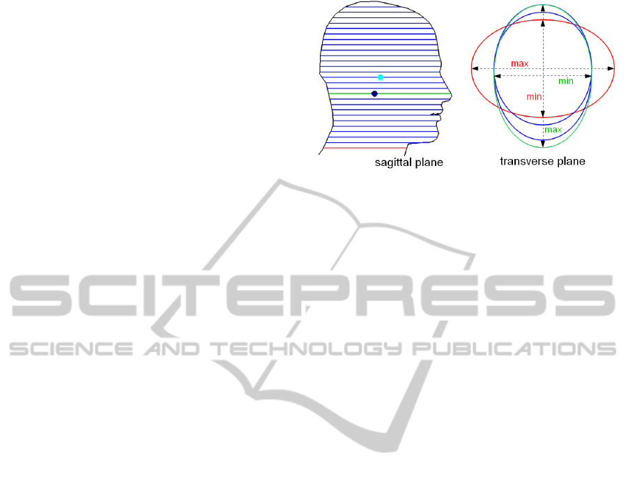
To compute the transverse body plane we use the
roughly aligned skeleton as follows. For each leg we
determine a vector pointing from the ankle to the hip.
Assuming an upright standing human, the average of
these vectors provides a reasonable approximation of
the normal of the transverse plane. Now we can ex-
tract the head’s geometry as a set of horizontal slices
by intersecting the mesh with a sequence of planes
parallel to the transverse plane, starting at the topmost
point of the mesh (fig. 1, left). Because of the varying
head sizes across all humans, the termination criterion
Figure 1: Termination criteria for head extraction (green:
maximal slice). Chin-throat transfer marked by decrease
in slice diameter (left) and head-torso transfer marked by
switching principal axes (right).
for this head extraction process cannot be based e.g.
on the body’s height. Instead we proceed as follows.
For each intersection polygon representing a slice we
employ a principal component analysis to its vertices
to compute the slice’s diameter as the maximum ex-
pansion along its major axis. During the extraction
process we keep track of the slice with the maximal
diameter and check if either the diameter of the cur-
rent slice has shrinked significantly compared to this
maximal slice (fig. 1, left), or if it’s principal axes
have rotated by 90
◦
compared to the maximal slice
(fig. 1, right). The former case marks the transfer
from chin to throat and the latter case marks the trans-
fer from head to torso in general and is only needed if
the former was not significant enough to be detected.
From the head geometry we can finally compute
the other two body planes as follows. After project-
ing all the head slices’ vertices into a single trans-
verse plane, both plane normals can be computed as
the principal axes of those points. Here we make use
of the assumption that the human is looking straight
ahead and that the head is longer in the forward di-
rection than in the sideward direction, which is less
restrictive than assuming a completely symmetrical
pose of the whole body. Furthermore, the head’s ge-
ometry can now be used to compute its centroid by
simply taking the perimeter-weighted average of the
slices’ centroids.
But what we are really looking for is the position
of the joint connecting the head with the spine (fig.
1, left, dark blue), which is not identical to the head’s
centroid (fig. 1, left, light blue). This joint is normally
at the height of the nose, so we first project the cen-
troid onto the plane corresponding to the slice with the
largest forward extent (fig. 1, left, green). Now only
its position inside the transverse plane needs to be ad-
justed slightly. By looking at a real skull cut along the
transverse plane (fig. 2, right), we see that the back
GRAPP 2012 - International Conference on Computer Graphics Theory and Applications
342

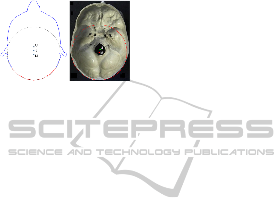
Figure 2: Joint position (J) as average of projected head
centroid (C) and occipital center (M) for head slice (left)
and real skull (right) (Crimando, 1998).
of the head is quite circular, with the circle’s center
lying near the searched joint position. Based on our
observations we approximate the back of the head by
a circle and compute the final joint position as the av-
erage of the projected head centroid and this circle’s
center point (fig. 2, left). The leaf node of the head
skeleton is only used to define the skull segment and
does not have an anatomical correspondence. Assum-
ing an upright head position, it is just set to the head
joint’s position, translated to the cranial roof along the
transverse plane’s normal.
3.2 Positioning of Spinal Joints
Despite its complicated anatomical structure, the ba-
sic shape of the spine can be described by a planar
curve in the median plane, the sagittal plane through
the center of the torso. This curve consists of four
parts with alternating signs of curvature (fig. 3a).
From top to bottom these parts consist of the 7 ver-
tebrae of the cervical spine, the 12 vertebrae of the
thoracic spine, the 5 vertebrae of the lumbar spine,
and the remaining 9 to 10 vertebrae that merged into
sacrum and coccyx over time. In the following we
will describe the steps for correctly positioning a
complete set of vertebral joints, meaning the abstract
joints connecting all 24 adjacent vertebrae of the up-
per three parts of the spine. In addition to this we also
compute the center point of the sacrum as a represen-
tation of the sacroiliac part of the spine.
By observing real humans it becomes evident that
the shape of the back quite closely follows the shape
of the spine (fig. 3b). In conjunction with the char-
acteristic shape of the spine curve this suggests to
create the curve by deducing its points of maximal
curvature from their corresponding points on the back
curve and interpolating these by a simple spline curve
(fig. 3c). A similar approach can be found in (Dellas
et al., 2007) to extract a simple 3-segment spine, but
we will take this idea further to extract the complete
set of spinal joints.
First we reduce the problem domain to two dimen-
sions by intersecting the mesh with the median plane.
This results in a closed polygon which we refer to
as the silhouette of the torso (fig 3c). To get a con-
tinuous representation of this silhouette and to cope
with low-polygon meshes, the vertices of this piece-
wise linear curve are interpolated by a cubic B-spline
curve, which gives a better approximation of the hu-
man shape.
Now we can extract some of the characteristic
points of the torso. For this we split the silhouette
at its lowest and highest points into a front and a back
segment. For both segments we consider the signed
distance function to the frontal plane, whose normal
points forward. Now, on the back segment we de-
fine the neck point and lumbar point as local max-
ima of this function and the back point and sacroiliac
point as local minima. For the front segment only the
throat as point of minimal distance to the frontal plane
and height between back and neck is of interest. The
crotch is simply marked by the lowest point on the
whole silhouette.
From these characteristic points, which are also
shown in fig. 3c (blue), corresponding points on the
spine curve (red) can be determined as follows. The
joint connecting the spine with the head — computed
in the previous section — represents the upper end
of this curve. The center of the throat as the aver-
age of the throat and neck points is also passed by the
spine and marks the beginning of the cervical spine
and, therefore, the joint between C7 and T1. The
back and lumbar points directly correspond to spe-
cific inter-vertebral joints on the same vertical posi-
tion, namely the joints connecting T6 with T7 and L3
with L4 respectively, moved from the back into the
body. The amount of this movement is just a heuristi-
cal value depending on the body’s overall height. The
height of the sacroiliac point marks the center point of
the sacrum and, together with the height of the crotch,
determines the lower end of the spine curve. Once
all these points have been computed, they are interpo-
lated by a Catmull-Rom spline, to yield the final spine
curve.
The remaining spinal joints’ positions along the
curve are determined in analogy to the size changes
of the vertebrae of a real spine, by minimizing the
length deviation of adjacent segments (fig. 3c). The
use of a chordal parameterization for the spine curve
and it’s rather simple shape — that stays quite close
to it’s control polygon — lets us treat the parame-
ter values as a reasonable approximation of the arc
ANATOMICALLY CORRECT ADAPTION OF KINEMATIC SKELETONS TO VIRTUAL HUMANS
343

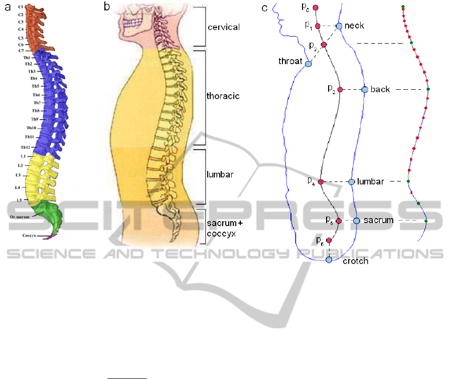
Figure 3: a) Different regions of a real spine. b) Spine with its shape closely following the back of a real human. c) Extracted
spine curve for virtual human with the characteristic points guiding its construction and the final positions of the spinal joints
along the curve.
length along the curve. Therefore, the positioning of
the spinal joints along the curve, represented by their
parameter values, can be computed by minimizing the
function
f (t) =
n−1
∑
i=2

t
i
−
t
i−1
+t
i+1
2

2
(1)
with t
i
being the parameter of the ith inter-vertebral
joint, which stays fixed for the joints corresponding
to the spine curve’s control points. Under the above
made assumptions for the parameter values this min-
imization strives for a joint distribution with adjacent
vertebrae having the same size.
3.3 Segmentation and Fitting of the
Limbs
Although not completely anatomically correct, it is
reasonable to assume the limbs’ joints lying on their
center lines. So the first step is to find the centroid
curves for the the legs and arms, together with some
more parameters describing their geometry. For this
we employ the Plumber algorithm developed in (Mor-
tara et al., 2004). This method extracts tubular parts
— in our case the limbs — as a sequence of slices
(fig. 4a), by repeatedly intersecting the geometry with
spheres. In contrast to the original Plumber method
we use the pre-aligned skeleton to define the start-
ing point of this extraction process. For each slice
the barycenter of the polygonal intersection curve,
its length, and its principal diameters are computed.
These barycenters are interpolated by a cubic B-spline
(fig. 4a), and to gain a continuous representation of
the limb’s geometry the lengths and diameters are also
interpolated by cubic B-splines, using the same pa-
rameterization as for the centroids.
For the positions of the hips we actually do not
need this information, as they can be deduced quite
easily from the previously computed characteristic
points of the torso. First, their height is taken as
the average of the heights of the crotch and sacroiliac
points. Next, we intersect the mesh with a transverse
plane at this height and use the centroids of the left
and right halves of the resulting intersection curve for
the hip joints’ positions (fig. 4b).
Despite their similarity the shoulders have to be
treated differently from the hips because of their much
higher flexibility. Although their height can also be
deduced from the spine, intersecting such a transverse
plane with the direction of the upper arm would be
very imprecise if the arms had a quite horizontal pose.
Instead of this, we first search the armpit as an in-
dicator for the shoulder position. Because it marks
the connection of the arm to the torso, this is a very
GRAPP 2012 - International Conference on Computer Graphics Theory and Applications
344

(a) (b) (c)
Figure 4: a) Computation of hip joints (blue) by intersecting the mesh with transverse plane at the height between crotch and
sacroiliac points (red). b) Computation of shoulder joint (blue) by 1. determining armpit point (red) on armpit curve and 2.
intersecting sagittal plane through armpit (dashed) with arm direction.
prominent geometrical feature and rather independent
of the model’s tessellation quality and posture. So we
first find the armpit as a distinct point of high curva-
ture (fig. 4c, red) on a surface curve running on the
side of the body in the frontal plane. Now we deter-
mine the upper arm direction by approximating the
upper part of the arm’s centroid curve by a line and
compute a sagittal plane through the armpit (fig. 4c,
dashed line), half-way rotated into the arm direction.
The intersection point of this plane with the approxi-
mated arm direction marks the shoulder position (fig.
4c, blue).
Because of its low flexibility, the ankle joint’s po-
sition can be found by simply searching for a point
of maximal curvature in the lower part of the leg’s
centroid curve (fig. 4a). Their arm counterparts, the
wrist joints, again have to be found differently. The
wrist joint marks a local minimum of the arm’s thick-
ness (measured from top to bottom) as well as a global
minimum of the arm’s width (measured from side to
side). In the region of the wrist these values fortu-
nately correspond to the previously computed princi-
pal diameters of the arm. So under all of the local
minima of the thickness — under which could also
be the palm — we use the one nearest to the global
minimum of the width, or more accurately, its corre-
sponding point on the arm’s centroid curve.
The knee and elbow joint can be found in a similar
way as the points on the middle parts of their respec-
tive limbs’ centroid curves, that produce the smallest
knee and elbow angles. If this joint position produces
a very obtuse angle we instead take the point produc-
ing the optimal upper to lower limb ratio proposed in
(Dellas et al., 2007) and search for a point with a slice
of minimal perimeter in its vicinity (fig. 4a).
4 RESULTS
After carrying out the described joint positioning pro-
cesses we have a detailed skeleton, adapted to the
geometric model of a human (fig. 5). For the left
model in fig. 5 we can compare the automatically
computed skeleton to a reference skeleton, which was
fitted manually by an expert in biomechanics. The av-
erage and maximum differences in joint position over
all optimized joints, compared to this reference skele-
ton, are 14 mm and 29 mm respectively, which shows
the accuracy of our methods.
By comparing the fitting results for differently
detailed versions of the same model (from 3,000 to
81,000 triangles) to the results on the version with
11,000 triangles (tab. 1), we see that the average
differences in joint position are at maximum 5 mm,
which shows the algorithms’ independence from the
overall tessellation quality of the meshes. But it
has to be noted, that the geometry analyses, espe-
cially the spine recognition, might be distorted by too
loose-fitting clothes, possibly requiring manual ad-
justments.
In fig. 6 we can see a very roughly aligned skele-
ton and the final result of our adaption based on this
pre-alignment. The apparent high quality of the align-
ment is due to the fact that the input skeleton is actu-
ally only used to guide the segmentation of the leg
and arm geometries. This figure also shows the pose
Table 1: Average differences in joint position for differently
tessellated versions of the same model, compared to the re-
sults obtained on a model with 11,000 triangles.
#∆ 6k 19k 32k 49k 81k
ε in mm 3.54 0.72 1.30 4.04 5.06
ANATOMICALLY CORRECT ADAPTION OF KINEMATIC SKELETONS TO VIRTUAL HUMANS
345

Figure 5: Skeleton fitting results for different human models.
independence of the proposed approach, as the aver-
age difference in segment length compared to the un-
deformed model’s skeleton is only 9 mm. But this
pose independence has its limits as the torso has to be
upright, for the spine recognition not to fail. And in
this particular case the body frame had to be specified
manually because the model neither stands on both
legs nor looks straight forward.
The fact that the skeleton fitting did not take
longer than half a second (measured on a Pentium 4
with 3 GHz) for all tested models, which had up to
81,000 triangles, is sufficient to show its efficiency,
assuming an absent real-time requirement anyway.
To finally use the skeleton for animating the mesh
there still needs to be made a connection between both
by computing the segments’ influences on the ver-
tices. This can be achieved by the method presented
Figure 6: Left: very rough skeleton alignment (based on
(Poirier and Paquette, 2009)). Right: optimized skeleton
based on this pre-alignment.
in (Baran and Popovi
´
c, 2007). Together with the pre-
alignment of (Lu et al., 2009) or (Poirier and Paque-
tte, 2009) and the proposed joint optimization we get
a nearly automatic pipeline for making an arbitrary
human model animation-ready.
REFERENCES
Baran, I. and Popovi
´
c, J. (2007). Automatic rigging and ani-
mation of 3d characters. ACM Transactions on Graph-
ics, 26(3):72.
Cornea, N. D., Silver, D., and Min, P. (2007). Curve-
skeleton properties, applications, and algorithms.
IEEE Transactions on Visualization and Computer
Graphics, 13(3):530–548.
Crimando, J. (1998). Skull anatomy tutorial.
Dellas, F., Moccozet., L., Magnenat-Thalmann, N., Mor-
tara, M., Patan
´
e, G., Spanguolo, M., and Falcidieno,
B. (2007). Knowledge-based extraction of control
skeletons for animation. In SMI ’07: Proceedings of
the IEEE International Conference on Shape Model-
ing and Applications 2007, pages 51–60.
Lu, L., L
´
evy, B., and Wang, W. (2009). Centroidal voronoi
tessellations for line segments and graphs. Technical
report, INRIA - ALICE Project Team.
Mortara, M., Patan
`
e, G., Spagnuolo, M., Falcidieno, B., and
Rossignac, J. (2003). Blowing bubbles for multi-scale
analysis and decomposition of triangle meshes. Algo-
rithmica, 38(1):227–248.
Mortara, M., Patan
`
e, G., Spagnuolo, M., Falcidieno, B., and
Rossignac, J. (2004). Plumber: a method for a multi-
scale decomposition of 3d shapes into tubular primi-
tives and bodies. In SM ’04: Proceedings of the ninth
ACM symposium on Solid modeling and applications,
pages 339–344, Aire-la-Ville, Switzerland.
Poirier, M. and Paquette, E. (2009). Rig retargeting for 3d
animation. In GI ’09: Proceedings of Graphics Inter-
face 2009, pages 103–110, Toronto, Ont., Canada.
GRAPP 2012 - International Conference on Computer Graphics Theory and Applications
346