SOUND LOCALIZATION USING COMPRESSIVE SENSING
Hong Jiang, Boyd Mathews and Paul Wilford
Bell Labs, Alcatel-Lucent, 700 Mountain Ave, Murray Hill, NJ 07974, U.S.A.
Keywords: Sound Localization, Compressive Sensing, Sparse Signal.
Abstract: In a sensor network with remote sensor devices, it is important to have a method that can accurately localize
a sound event with a small amount of data transmitted from the sensors. In this paper, we propose a novel
method for localization of a sound source using compressive sensing. Instead of sampling a large amount of
data at the Nyquist sampling rate in time domain, the acoustic sensors take compressive measurements
integrated in time. The compressive measurements can be used to accurately compute the location of a
sound source.
1 INTRODUCTION
This paper is concerned with localization of sound
source in a network of distributed acoustic sensors.
In a typical application of wireless distributed
sensing network for surveillance, acoustic sensors
are distributed remotely in a region of interest. Each
sensor collects samples of sound wave arrived at its
location from a sound source. The sensors transmit
the collected samples to a processing center where
the samples are analyzed and the location of the
sound source is estimated and tracked. The sensors
are small, low-cost devices that may be powered by
batteries. Each sensing device integrates the
functionality of converting acoustic pressure to an
electronic signal, sampling the electronic signal and
transmitting the samples via wireless
communications. In such a scenario, it is important
for the sensors to be built with high reliability, low
complexity and low power consumption. The best
way to achieve all these is to reduce the sampling
rate required at the sensing devices. A low sampling
rate at the sensors not only reduces the complexity
of the devices but also significantly reduces power
consumption of the circuits used for both analog to
digital conversion (ADC) and the wireless
transmission. A low rate wireless transmission also
increases reliability of the data transmission.
The Nyquist sampling rate of the acoustic
sensing devices is determined by the frequency
range that is needed in an application. For
localization of sound sources, the sampling rate
needs to be high enough to cover the acoustic
frequency range that is necessary to perform
localization with a prescribed resolution and
accuracy. Most sound localization techniques are
based upon determining the difference in
propagation time for a signal emitted from a source
to arrive at two or more sensors. This is known as
the time-difference-of-arrival (TDOA). In these
techniques, sound waves are sampled at the Nyquist
sampling rate by the sensors, and then TDOA is
determined from the collected samples. The cross-
correlation method (Knapp and Carter, 1976, Valin,
Michaud, Rouat and L´etourneau, 2003) uses the
location of the peak value in the sample cross-
correlation between two sensors to estimate TDOA.
Other methods (Benesty, Chen and Huang, 2008)
make use of channel response functions of the
signals arrived at the sensors.
Compressive sensing (Candès, Romberg and
Tao, 2006) is an emerging theory for representing
and reconstructing sparse signals by using far fewer
measurements than the number of Nyquist samples.
When a signal has a sparse representation, the signal
may be reconstructed from a small number of
measurements from linear projections onto some
basis. Furthermore, the reconstruction has high
probability of success even if a random sensing
matrix is used.
In this paper, we develop a method for sound
localization in a distributed sensing network using
compressive sensing. In order for localization to be
reliable for a variety of sound events, we don’t make
the assumption that the sound wave from a sound
159
Jiang H., Mathews B. and Wilford P..
SOUND LOCALIZATION USING COMPRESSIVE SENSING.
DOI: 10.5220/0003822301590166
In Proceedings of the 1st International Conference on Sensor Networks (SENSORNETS-2012), pages 159-166
ISBN: 978-989-8565-01-3
Copyright
c
 2012 SCITEPRESS (Science and Technology Publications, Lda.)

source is sparse. Instead, we observe that in most
reasonable circumstances, the acoustic signal at one
sensor has a sparse representation if the acoustic
signal at another sensor is known. We regard the
signal at one sensor to be the output of a linear
system with the input as the signal at another sensor,
and we assume that the linear system can be
approximated by a finite impulse response filter with
a very small number of nonzero coefficients.
Consequently, it is possible for sensors to take and
transmit very small number of measurements if the
signal at one of the sensors is known.
By using compressive measurements, a sound
sensor is only required to make and transmit samples
at a low rate, which improves the reliability of the
sensor and reduces the power assumption.
Furthermore, since the measurements are made by
linear projections, the complexity of acquiring the
measurements is also low.
The paper is organized as follows. In section 2,
we describe existing sound localization techniques.
Our method of localization using compressive
sensing is described in Section 3. Some simulation
and experiment results are presented in Section 4,
and the conclusion is provided in Section 5.
2 SOUND LOCALIZATION
TECHNIQUES
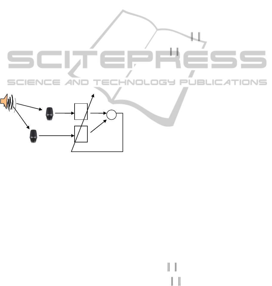
Figure 1 illustrates a distributed sensor network. The
sensors are distributed with a known geometry. The
sensors make samples of the sound waves, and
transmit the samples to a processing center (not
shown) for analysis.
2.1 Direction of Arrival (DOA) and
Time Difference of Arrival (TDOA)
The location of the sound source can be estimated
from the time differences between the arrival times
of the sound wave at the sensors. For the purpose of
this paper, we consider the case where the sound
source is sufficiently distant so that the wavefront
arriving at the array approximates a plane. Figure 1
shows the derivation of the DOA shown as angle θ
between the segment
10
xx and the arriving sound.
The quantity d
1
cos(θ) can be calculated by
measuring the time delay, τ
01
, for the wavefront to
propagate from x
0
to x
1
. Using c to denote the
velocity of sound in air, we have
(
)
θ
τ
cos
101
dc =
,
and thus
()
101
1
cos dc τθ
−
=
. In this way, a pair of
sensors can be used to determine the relative
direction to the sound source. Multiple pairs can be
used to triangulate upon the source position.
Sound
sensors
x
1

x
0
x
2
d
1
d
2
Sound
source
θ
d
1
cos(θ)
Figure 1: Distributed sensor network.
2.2 Cross-correlation
Cross-correlation of the sensor signals, proposed by
(Knapp, Carter 1976) is the most straightforward
means to measure TDOA. Given a single sound
source in a quiet anechoic space, the output of each
sensor is a transduction of the source signal affected
only by the delay and attenuation associated with the
path length between the source and sensor. The
cross-correlation of two such signals is maximized
at the time lag corresponding to the difference in
path delays. Let
)(
0
ix and )(
1
ix represent the
samples of signals arriving at sensors x
0
and x
1
. The
samples are processed in blocks of length N. For
each block of samples, we calculate the cross-
correlation function
∑
−
=
−=
1
0
2112
)()()(
N
i
ixixr ττ ,
where the range of τ is limited to
cd
max
≤
τ
by the
maximum distance between sensors. TDOA is
determined by finding the value of delay which
maximizes the cross-correlation
)(maxarg
τ
τ
τ
r
TDOA
=
.
Several aspects of cross-correlation for TDOA
estimation should be noted. First, correlation of
periodic signals is also periodic. Spatial aliasing will
occur for periodic signals with a wavelength shorter
than twice the sensor spacing. Also, even for non-
periodic signals, echoes can degrade the accuracy of
this method by creating local maxima in the cross-
correlation function.
The cross-correlation approach for TDOA
estimation is normally performed in the frequency
domain (Valin, Michaud and Rouat and
SENSORNETS 2012 - International Conference on Sensor Networks
160

L´etourneau, 2003) and many enhancements have
been proposed based upon frequency weighting
functions. The smoothed coherence (SCOT) method
(Carter, Nuttall and Cable, 1973) attempts to
minimize the influence of the source signal power.
The phase transform (PHAT) method (Knapp and
Carter, 1976) removes the source amplitude from
the cross-spectrum calculation altogether. However,
we will not elaborate further in this direction and
instead consider a quite different way of looking at
TDOA estimation.
2.3 Channel impulse Response
The adaptive eigenvalue decomposition (AED)
algorithm presented by (Benesty, Chen and Huang,
2008) measures TDOA between two sensors by
estimating the channel response from the source to
each sensor. The direct path feature is extracted
from each channel response and the timing
difference between these two features is taken as the
TDOA estimate.
h
0

h
1

Σ
1
ˆ
h

0
ˆ
h

‐
+
erro
r
s
x
1

x
0

Figure 2: Adaptive estimate of channel responses.
As illustrated in Figure 2, given the source
signal, s, is not known, the fundamental observation
allowing estimation of the two channel responses is
0**
1001
=− hxhx
TT
.
A constrained LMS algorithm, presented in
(Benesty, Chen and Huang, 2008), can be
formulated allowing adaptation towards the
concatenated channel response estimates
0
ˆ
h
and
1
ˆ
h
. After convergence, the maximum amplitude of
each response is assumed to correspond to the
arrival of the direct sound and the time difference
between these peaks is the TDOA. A significant
advantage of AED over cross-correlation is its
robustness under reverberant conditions.
3 LOCALIZATION USING
COMPRESSIVE SENSING
3.1 Compressive Sensing Background
A brief review of compressive sensing is given in
this subsection. A signal
N
x ℜ∈ is sparse if it is
comprised of only a small number of nonzero
components when expressed in certain basis
(Candès, Romberg and Tao, 2006). Specifically,
x
is
S -sparse if there exists an invertible matrix
NN ×
ℜ∈
ψ
and a vector
N
h ℜ∈
such that
hx
ψ
=
, and NSh <<=
0
.
(3.1)
In (3.1),
0
h
is the number of nonzero elements
of
h .
Since
h has S nonzero elements, signal
x
can
be uniquely represented by no more than
S2
numbers in a straightforward way: the locations and
the values of the nonzero elements of
h . However,
this representation requires the availability of all
N
samples of signal
x
. In other words, this
representation still requires the signal
x
to be
acquired with
N
samples.
Compressive sensing makes it possible to
acquire a sparse signal using far fewer than
N
measurements. In compressive sensing, a signal is
projected onto a measurement basis, and the
projections can be used to recover the signal.
Specifically, let
NM ×
ℜ∈ φ be a sensing matrix.
Then the measurements
M
y ℜ∈ are given by
xy
φ
=
.
(3.2)
The number of measurements
M
can be much
smaller than the length of vector
x
,
N
. Under the
conditions that 1)
φ
and
ψ
are incoherent; and 2)
M
is large enough with respect to S (Candès,
Romberg and Tao, 2006), the sparse signal
x
can
be reconstructed from the measurements
y
by
solving the following minimization problem:
1
min h subject to
yh =
φ
ψ
.
(3.3)
In (3.3),
1
h is the sum of the absolute values
of the components of
h . After h is found from
(3.3),
x
is computed from hx
ψ
= . The
SOUND LOCALIZATION USING COMPRESSIVE SENSING
161

minimization problem (3.3) can be solved by using
standard linear programming techniques.
Although it is difficult to verify the incoherence
condition for given sensing matrix
φ
and sparsity
basis
ψ
, it is known (Candès, Romberg and Tao,
2006) that for a given sparsity basis
ψ
, a random
sensing matrix
φ
has a high probability of being
incoherent with
ψ
. In other words, the signal
x
has a high probability of being recovered from
random measurements. In practice, it has been found
that randomly permutated rows of the Walsh-
Hadamard matrix may be used to form a sensing
matrix with satisfactory results (Li, Jiang and
Wilford and Zhang, 2011, Jiang, et al., 2012).
Sensing matrix formed from shifted maximum
length sequence (MLS) will be discussed later.
3.2 Sound Localization
We now describe our method for performing sound
localization by using compressive sensing.
As shown in Figure 1, let
)(ts represent the
acoustic signal from the sound source, and
)(
)(
tx
i
represent the signal of the sound source arriving at
the sensor
i
. Then signal
)(
)(
tx
i
can be written as
()
()( )
() () ()
() ()
0
ˆ
ˆ
() * ()
ˆ
ˆ
().
iii
t
ii
xt h s t
hstd t
η
τττη
=+
=−+
∫
(3.4)
In Eq. (3.4),
)(
ˆ
)(
th
i
is the impulse response of the
channel from the sound source to sensor
i , and
)(
ˆ
)(
t
i
η is the Gaussian noise.
We assume that the channel from the sound
source to sensor
0=i is invertible, i.e., there is a
deconvolution of
)(
)0(
tx so that
(
)
)()(*)(
)0()0(
ttxgts η += .
(3.5)
Then Eqs (3.4) and (3.5) give rise to the following
equations
(
)
() ( )
() () (0) ()
() (0) ()
0
() * () (),
( ),
1,2,...
ii i
t
ii
xt h x t t
hxtd t
i
η
τττη
=+
=−+
=
∫
(3.6)
where
() () () () (0)
ˆ
ˆ
ˆ
*, * ,
1, 2,...
iiii
hgh g
i
η
ηη ==−
=
(3.7)
Equations in (3.6) and (3.7) show that if a
deconvolution of
)(
)0(
tx
exists, then each signal
arriving at the other sensors
)(
)(
tx
i
,
,...2,1=i
, is a
convolution of
)(
)0(
tx
plus noise.
Let us now consider the discrete samples of the
acoustic signals with sample duration of
T
. Let
Ni
x ℜ∈
)(
,
)(i
n
x ,
Nn ,...,0
=
be the samples of the
signal
)(
)(
tx
i
, and
Nnhh
i
n
Ni
,...,0,,
)()(
=ℜ∈
be
the samples of
)(
)(
th
i
. For convenience, although it
is not necessarily, we assume that
N
is an even
number.
We assume that the number of samples
N
is
large enough so that the support of
)(
)(
th
i
is
contained within the interval
],0[ NT
, that i.e.,
],0[,0)(
)(
NTtth
i
∉= , ,...2,1=i
(3.8)
Eq. (3.8) may not be satisfied for any finite
N
if the signal at sensor
0
=
i contains echoes. This is
because even though
)(
ˆ
)(
th
i
and
)(
ˆ
)0(
th
may have a
finite support, the deconvolution
)(tg
, and hence
)(
ˆ
*)()(
)()(
thtgth
ii
=
may not. Nevertheless, the
amplitude of
)(
)(
th
i
outside of the interval
],0[ NT
can be made small enough to be ignored for
sufficiently large
N
so that it is reasonable to
assume Eq. (3.8) holds in practice for large
N
.
The discretized version of Eq. (3.6) becomes
,...2,1 ,
)()(
0
)(
=+= ihx
iii
ηψ
(3.9)
where
.
,,
)0(
2
3
)0()0(
2
)0(
2
)0(
0
)0(
2
0
)(
)(
0
)(
)(
)(
0
)(
⎥
⎥
⎥
⎥
⎦
⎤
⎢
⎢
⎢
⎢
⎣
⎡
=
⎥
⎥
⎥
⎦
⎤
⎢
⎢
⎢
⎣
⎡
=
⎥
⎥
⎥
⎦
⎤
⎢
⎢
⎢
⎣
⎡
=
−
NNN
NN
i
N
i
i
i
N
i
i
xxx
xxx
h
h
h
x
x
x
LL
MOMOM
LL
MM
ψ
(3.10)
The vectors
)(i
h ,
,...2,1
=
i
, are sparse because most
of its entries are zero or small. The entries of
)(i
h
with largest absolute values provides information on
SENSORNETS 2012 - International Conference on Sensor Networks
162

the time delay between signals
)(
)(
tx
i
and
)(
)0(
tx .
For example, if the time delay between
)(
)(
tx
i
and
)(
)0(
tx is an exact integer multiple of the
sample duration
T
, then the time delay between the
two signals is given by
{}
T
N
ht
i
j
j
i
⎟
⎠
⎞
⎜
⎝
⎛
−=Δ
2
maxarg
)()(
.
(3.11)
Time delay of a fraction of sample duration may
be obtained by interpolation using a few
neighboring values of the entry with maximum
absolute value.
Eq. (3.9) shows that
)(i
x is a sparse signal with
sparsity basis
0
ψ
. Note that no assumption has been
made regarding the sparsity of the acoustic source
signal
)(ts . Regardless of whether or not the source
signal
)(ts is sparse, the signal
)(i
x
sampled at
sensor
,i
,...2,1=i , always has a sparse
representation in the basis
0
ψ
after
)0(
x
is
available. Therefore, the theory of compressive
sensing may be directly applied to the sparse signals
)(i
x , ,...2,1=i
Let
NM
i
×
ℜ∈ φ be the sensing matrix at sensor
i . Each of the sensors ,i ,...2,1=i takes
measurements
Mi
i
i
xy ℜ∈=
)()(
φ .
(3.12)
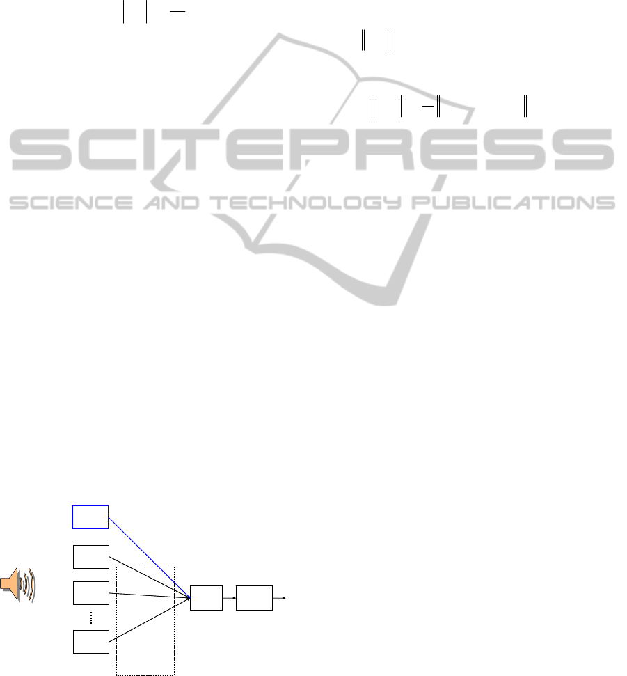
However, sensor
0=i takes samples
)0(
x of the
sound wave in the traditional way using the Nyquist
sample rate. This entire process is shown in Figure
3.
Sound
sensor 1
Sound source
Processing
device
Sound
sensor 2
Sound
sensor K
Relative
time delays
Compressive
measurements
)1(
n
y
)2(
n
y
)(K
n
y
Sound
sensor 0
)0(
n
x
Samples with high sample rate
Sound
sensor 1
Sound source
Processing
device
Sound
sensor 2
Sound
sensor K
Relative
time delays
Compressive
measurements
)1(
n
y
)2(
n
y
)(K
n
y
Sound
sensor 0
)0(
n
x
Samples with high sample rate
Figure 3: Distributed sensing network with compressive
sensing.
In Figure 3, a network of 1+
K
sound sensors is
shown. The sensors are configured so that one
sensor takes the traditional Nyquist samples, but the
other
K
sensors make compressive measurements.
In order to compute the time deference between
)(i
x
and
)0(
x
, the Nyquist sampled signal
)0(
x
is
used to form the sparsity basis
0
ψ
by using Eq.
(3.10). Then the channel response
)(i
h is computed
from the minimization problem
,min
1
)(
)(
i
h
h
i
subject to
)()(
0
ii
i
yh = ψφ
,
(3.13)
or, in practice
⎭
⎬
⎫
⎩
⎨
⎧
−+
2
)()(
0
1
)(
2
min
)(
ii
i
i
h
yhh
i
ψφ
μ
(3.14)
In (3.14),
0>
μ
is a constant.
3.3 Implementation Considerations
We discuss some practical issues of implementation
in this subsection.
Sensing matrix
The sensing matrix
φ
may be formed from a
maximum length sequence (m-sequence). M-
sequences have been traditionally used in audio
processing (Rife and Vanderkooy, 1989), but they
are used for a different purpose in this context. Let
Nnp
n
,...,1,
=
be a binary m-sequence generated
from a primitive polynomial. Then each row of the
sensor matrix
φ
is formed by a shifted sequence of
n
p . For example the entries of the sensor matrix
can be defined by
()mod
12 ,
1,..., , 1,...,
ij j i N
p
iM
j
N
φ
+
=
−
==
,
(3.15)
The advantage of using the shifted m-sequences
to form the sensor matrix is that the m-sequence can
be easily implemented in hardware by using linear
feedback shift registers and hence reducing the
complexity of matrix generation in the sensors.
All sensors need not use the same sensing
matrix. However, different sensing matrix can be
created with the same m-sequence, but with
different shifts for the rows. Again, this arrangement
helps reducing complexity.
SOUND LOCALIZATION USING COMPRESSIVE SENSING
163

Detection confidence indicator
The solution to minimization problem (3.14) has a
stochastic nature. This can be viewed from two
aspects. First, when a random sensing matrix such as
(3.15) is used, the compressive sensing theory only
guarantees the success of recovery with a high
probability. Therefore, the peak value in the solution
to (3.14) only provides the correct time delay in the
statistical sense. Secondly, the solution to (3.14) is
only meaningful when there is a sound from the
source. For example, the signals at the sensors are
comprised of only noise when the source is silent,
and the solution to (3.14) would result in a peak at a
random location.
The stochastic nature can be exploited to our
advantage to create a metric of how accurate the
solution is. In other words, we are able to utilize the
characteristics of compressive sensing to create an
indicator on how confident we are about the
detection of the sound source.
When
M
measurements
)(i
y are received from
sensor
i , they are used in (3.14) to compute an
estimate of the time delay
)(i
tΔ as given by Eq.
(3.11). Similarly, any subset of the measurements
may also be used to repeat the process. Therefore,
the minimization process (3.14) may be performed
multiple times, each time with a randomly selected
small number of measurements removed from
)(i
y ,
to compute multiple estimates of the time delay
)(i
j
tΔ . Here the subscript
j
denotes the repetition
index of process (3.14) for the estimate of the same
time delay
)(i
tΔ . The values of
)(i
j
tΔ
,
,...,1=j
may
be processed to produce a final estimate
)(i
tΔ and a
metric of confidence
)(i
C
. For example, they may
be defined as
}{min}{max
1
},{median
)()(
)(
)()(
i
j
j
i
j
j
i
i
j
j
i
tt
C
tt
Δ−Δ
=
Δ=Δ
(3.16)
Since these computations are done at a processing
center, not at the sensors, the complexity is not a
concern.
4 SIMULATION AND
EXPERIMENT
We present some simulation and experiment results
in this section.
4.1 Simulation with Three Sensors
In this simulation, the sensing network consists of
three sensors as shown in Figure 4.
Sound sensors
dd
r
Sound source
c
v
Sound sensors
dd
r
Sound source
c
v
Figure 4: Moving sound source with three sensors.
The sensors are placed horizontally on the x-axis
with distance
d
. A sound source is moving with
speed
v in a circle of radius
r
with the center on
the y-axis and a distance of
c
away from the x-axis.
The sensor in the middle is chosen to take Nyquist
samples, i.e.,
0
=
i . The signal source is chosen
from (Lin, Lee and Saul, 2004) and given by the
equation
tfets
t
0
2
1
2sin)(
2
π
τ
⎟
⎠
⎞
⎜
⎝
⎛
−
= .
(4.1)
The following parameters are used in for the
model network of Figure 4.
sec1016/47.0
571
0
===
===
τ kHzfsmv
mrmcmd
(4.2)
The middle sensor,
0
=
i
, takes Nyquist samples
of the arriving sound signal at the sample rate of
kHzf
s
16
=
. The sensors at two sides,
2,1=i
, make
compressive measurements of the arriving signals.
The sensing matrix
φ
is formed from shifted m-
sequences as described in Section III. Each
measurement is a projection of
4095=N
samples
of
kHzf
s
16
=
. In other words, the estimate of time
delay is performed on blocks of
4095=N
samples,
which corresponds to a time duration of 0.256
seconds. For each block,
40=M measurements
are used in the minimization process (3.14). For
SENSORNETS 2012 - International Conference on Sensor Networks
164

each set of measurements from sensors
2,1
=
i
, the
solution to the minimization problem (3.14)
produces an estimate for the time difference of
arrival (TDOA) between the side sensor and the
middle sensor,
)(i
tΔ , by using Eq. (3.11). The
estimate is accurate up to the sample duration. The
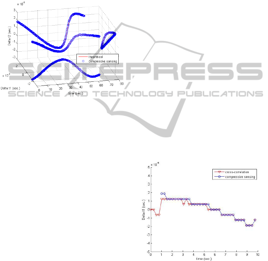
results of the time differences are shown in Figure 5.
Figure 5: Time differences at the sensors for a moving
sound source.
In Figure 5, the TDOA
)(i
tΔ ,
2,1=i
, are
plotted at different time instances. The x-axis in
Figure 5 is the time instances. The y- and z-axes are
for
)1(
tΔ
and
)2(
tΔ
, respectively. The sound source
moves at a constant speed in a circle, and it takes
about 66.3 seconds to complete the circle. As the
sound source moves along the circle, the pair of
TDOAs (
)1(
tΔ ,
)2(
tΔ ) traces out a loop in the
)2()1(
tt Δ−Δ plane that has a shape of a cloth
hanger. The computed result is compared to the
theoretical result, and the error in the computed
result is within one sample duration (
s
μ
5.62
) since
the resolution of the estimate as given in (3.11) is
the sample duration.
An important observation from this simulation is
that the result was achieved by using only
40
=
M
measurements for each of the side sensors
2,1
=
i
,
as opposed to the traditional Nyquist samples of
4095=N
. This represents a compression ratio of
more than 100 times. In other words, each of the
sensors
2,1=i
takes 40 measurements and
transmits them to the processing center, instead of
traditional 4095 samples. The compression ratio of
more than 100 times implies that the sensors are able
to transmit the measurements much more reliably
and power-efficiently. Also the compression ratio is
achieved with a very low complexity of projections
with the sensing matrix formed from the shifted m-
sequences.
4.2 Experiments with Two Sensors
In this subsection, we present two experiments with
data from actual recordings from two microphones.
In the experiments, two microphones are placed in a
room about 11 cm apart. The microphones are used
to make recordings of a person reading an article.
Signals from both microphones are sampled at the
same Nyquist sampling rate. The samples from one
microphone is used to form the sparsity basis
0
ψ
,
and the samples from another microphone is used to
form the compressive measurements using a random
sensing matrix formed by the shifted m-sequences.
The number of full samples is
4095=N
, and the
number of measurements is
40=M
, representing a
compression ratio of 100. The estimate of difference
in signal arrival times is computed by solving the
minimization problem (3.14), and the results are
compared to those obtained by using the classic
cross-correlation method by using the full
4095
=
N
samples.
In the first experiment, the setup is such that the
signals from the microphones are clean, and the
speaker remains relatively still. In this experiment,
the sample rate is
kHzf
s
16=
. The result, compared
with the cross-correlation, is shown in Figure 6.
Figure 6: Two sensors with clean signals.
At the start of the recording, there is a segment
of silence. As described in Section III, the
compressive sensing method is able to ignore the
results from that segment by using the confidence
indicator (3.16). The confidence indicator is much
SOUND LOCALIZATION USING COMPRESSIVE SENSING
165

less than 1 during the initial segment in which the
cross-correlation result is unreliable as well. After
the initial silent segment, the confidence indicator is
infinity and the result matches with the cross-
correlation very well.
In the second experiment, the setup represents a
difficult environment in which echoes and noise are
abundant. In addition, the speaker is constantly
moving around. The sample rate for this experiment
is
kHzf
s
1.44=
. The result, compared with the
cross-correlation, is shown in Figure 7.
This is a difficult situation as is evident by many
erroneous results from the cross-correlation method.
Admittedly, the compressive sensing method made
many erroneous calculations as well, but the use of
the confidence indicator is able to identify and
eliminate the unreliable data points. The eliminated
data points from compressive sensing are not plotted
in Figure 7, which can be seen from the connected
line without the symbol. It is worthwhile to point out
that it is possible to apply certain processing to
eliminate the erroneous results from the cross-
correlation method as well. However, the purpose of
showing the result from the cross-correlation
method without further processing is to illustrate
that the environment used in this experiment is a
difficult one, and even in this difficult environment,
the compressive sensing method is able to produce
reasonable result with a high compression ratio of
more than 100 to 1.
Figure 7: Two sensors with noisy signals.
5 CONCLUSIONS
Compressive sensing is an effective technique for
localization of sound source in a sensing network.
Compressive measurements can be used to reliably
estimate the time difference of arrival (TDOA) of
sound signals at the sensors, without any assumption
on the sparseness of the sound source. We have
demonstrated reliable detection and tracking of
sound source by using compressive measurements
with a compression ratio of more than 100 times, as
compared to the traditional Nyquist sampling.
REFERENCES
Knapp, C. Y., Carter, G. C., 1976, The generalized
correlation method for estimation of time delay, IEEE
Trans. Acoust. Speech, Signal Processing, vol. ASSP-
24, pp. 320-327.
Valin, J., Michaud, F, Rouat, J, L´etourneau, D., 2003,
Robust Sound Source Localization Using a
Microphone Array on a Mobile Robot, Proceedings of
2003 IEEE/RSJ International Conference on
Intelligent Robots and Systems (IROS 2003), vol.2, pp.
1228 – 1233.
Benesty, J., Chen, J., Huang, Y., 2008, Adaptive
Eigenvalue Decomposition Algorithm, Microphone
Array Signal Processing, pp. 207-208. Berlin,
Germany: Springer-Verlag.
Carter, G. C., Nuttall, A. H., Cable, P. G., 1973, The
smoothed coherence transform,” Proc. IEEE, vol. 61,
pp. 1497-1498.
Candès, E., Romberg, J., Tao, T., 2006, Robust
uncertainty principles: Exact signal reconstruction
from highly incomplete frequency information, IEEE
Trans. on Information Theory, vol 52, no 2, pp. 489-
509.
Rife, D. D., Vanderkooy, J., 1989, Transfer-Function
Measurement with Maximum-Length Sequences,
Journal of the Audio Engineering Society, vol 37, no
6, pp. 419-444.
Lin, Y., Lee, D. D., Saul, L. K., 2004, Nonnegative
deconvolution for the time of arrival estimation, IEEE
International Conference on Acoustics, Speech, and
Signal Processing, Proceedings. (ICASSP '04), vol 2,
pp. 377-380.
Li, C., Jiang, H., Wilford, P. A., Zhang, Y., 2011, Video
coding using compressive sensing for wireless
communications, IEEE Wireless Communications and
Networking Conference (WCNC), 10.1109/WCNC.
2011. 5779474, pp. 2077 – 2082.
Jiang, H. Li, C., Haimi-Cohen, R., Wilford, P., Zhang, Y.,
2012, Scalable Video Coding using Compressive
Sensing, Bell Labs Technical Journal, vol. 16, no. 4.
SENSORNETS 2012 - International Conference on Sensor Networks
166