DOWNSCALING AEROSOL OPTICAL THICKNESS TO 1 KM

SPATIAL RESOLUTION USING SUPPORT VECTOR REGRESSION

REPLIED ON DOMAIN KNOWLEDGE

Thi Nhat Thanh Nguyen

, Simone Mantovani

2,3

, Piero Campalani

and Gian Piero Limone

Department of Mathematics, University of Ferrara, Via Saragat 1, 44122, Ferrara, Italy

MEEO S.r.l., Via Saragat 9, 44122, Ferrara, Italy

SISTEMA GmbH, W

ahringerstrasse 61, A-1090, Vienna, Austria

Department of Engineering, University of Ferrara, Via Saragat 1, 44122, Ferrara, Italy

Keywords:

Aerosol optical thickness, Downscaling, 1 km

spatial resolution, Support vector regression, MODIS, Local

monitoring, Air pollution, Remote sensing.

Abstract:

Processing of data recorded by MODIS sensors on board the polar orbiting satellite Terra and Aqua usually

provides Aerosol Optical Thickness maps at a coarse spatial resolution. It is appropriate for applications of

air pollution monitoring at the global scale but not adequate enough for monitoring at local scales. Different

from the traditional approach based on physical algorithms to downscale the spatial resolution, in this article,

we propose a methodology to derive AOT maps over land at 1 km

of spatial resolution from MODIS data

using support vector regression relied on domain knowledge. Experiments carried out on data recorded in

three years over Europe areas show promising results on limited areas located around ground measurement

sites where data are collected to make empirical data models as well as on large areas over satellite maps.

1 INTRODUCTION

Remote Sensing allows to measure physical proper-

ties of objects without actually being in contact with

them. Using devices installed on board aircrafts or

satellite platforms, Remote Sensing applied to the

Earth Observation makes it possible to monitor the

Earth-Atmosphere system through the analysis of the

interaction of radiation with matter. The signal re-

ceived by satellite optical sensors is the sum of sev-

eral contributions due to scattering, absorption, reﬂec-

tion and emission processes. Image processing tech-

niques and speciﬁc algorithms are applied on that in-

formation to extract (direct measurement) or estimate

(indirect measurement) the environmental parameters

and their characteristics which are used in a large va-

riety of applications for Earth Observation (Agricul-

ture, Atmosphere, Forestry, Geology, Land Cover and

Land Use, Mapping, Oceans and Coastal).

For Atmosphere applications focused on the Cli-

mate Change and on the human health, the Aerosol

Optical Thickness (AOT) has been recognized as

one of the most important atmospheric variables to

be monitored from local to global scale. AOT is

representative for the amount of particulates present

in a vertical column of the Earth’s atmosphere.

Aerosol concentration can be measured directly by

ground-based sensors or estimated by processing data

recorded by airborne instruments or by satellite-based

sensors. Ground measurements have usually high

accuracy and temporal frequency (hourly) but they

are representative of a limited spatial range around

ground sites. Conversely, satellite observation pro-

vides information at global scale with moderate qual-

ity and lower measurement frequency (daily).

MODerate resolution Imaging Spectrometer

(MODIS) is a multispectral sensor on-board the two

polar orbiting satellites Terra and Aqua, launched

in 1999 and 2002, respectively and operated by

the National Aeronautic and Space Administration

(NASA). These satellite sensors provide observations

nearly the entire globe on a daily basis, and repeat

orbits every 16 days. MODIS sensors perform

measurements of sectorial radiances in the solar to

thermal infrared spectrum region from 0.41 to 14.235

µm. Using MODIS-measured spectral radiances,

physical algorithms based on Look-Up Table (LUT)

approaches have used since 90s to generate the

230

Nhat Thanh Nguyen T., Mantovani S., Campalani P. and Piero Limone G. (2012).

DOWNSCALING AEROSOL OPTICAL THICKNESS TO 1 KM2 SPATIAL RESOLUTION USING SUPPORT VECTOR REGRESSION REPLIED ON

DOMAIN KNOWLEDGE.

In Proceedings of the 1st International Conference on Pattern Recognition Applications and Methods, pages 230-239

DOI: 10.5220/0003791302300239

 SciTePress

aerosol products for Land and Ocean areas in Collec-

tion 004 (Kaufman and Tanre, 1997) and following

improved releases (Collection 005 (Remer et al.,

2004), Collection 051 and the newest Collection 006

issued in 2006, 2008 and 2012, respectively).

Over the Land areas, the aerosol optical thickness

is derived using the Dense Dark Vegetation (DDV)

approach. Firstly, all cloudy pixels are removed by

cloud scanning process. After that, dark pixels are

identiﬁed by low reﬂectance values in the mid in-

frared channel 2.13 µm. Reﬂectance in 0.645, 0.466,

and 2.13 µm over dark pixels are used to derive

the optical thickness in those three channels. For

the inversion process, in Collection 005, parame-

ters of different aerosol models consisting of Con-

tinental, Neutral/Generic, Non-absorb/Urban Indus-

try, Absorbing/Heavy Smoke, Spheroid/Dust mod-

els are calculated and stored in LUT. The algo-

rithm assumes that aerosol properties over a targeted

pixel are presented by proper weightings of one ﬁne-

dominated aerosol model and one coarse-dominated

aerosol model. Spectral reﬂectance from the LUT is

compared with MODIS-measured spectral reﬂectance

to ﬁnd the best match that is the solution to the inver-

sion process.

Machine learning approaches applied in aerosol

optical thickness processing have recently been in-

vestigated and presented in various applications rang-

ing from classiﬁcation of aerosol components (Ra-

makrishnan et al., 2005), prediction based on time

series data (Lu et al., 2002)(Osowski and Garanty,

2006)(Chen and Shao, 2008)(Siwek et al., 2008),

to estimation of aerosol content and properties from

different sensors (Okada et al., 2001)(Han et al.,

2006). Related to MODIS aerosol retrievals, pro-

posed approaches often follow a general frame-

work that applies machine learning techniques on

data collected by different instruments. Firstly, in-

tegrations of ground-based measurements AErosol

RObotic NETwork (AERONET) and data recorded

by satellite sensors (Multi-angle Imaging SpectroRa-

diometer (MISR) and MODIS (Xu et al., 2005) or

only MODIS (Vucetic et al., 2008)(Lary et al., 2009)

are made. After that, Neural Networks (NNs) or Sup-

port Vector Regression (SVR) techniques are applied

on integrated data to derive aerosol content and prop-

erties. This method proved efﬁciency in reducing pro-

cessing time (Okada et al., 2001), dealing with data

uncertainties (Vucetic et al., 2008)(Obradovic et al.,

2010), improving estimation accuracy (Xu et al.,

2005)(Vucetic et al., 2008)(Nguyen et al., 2010b),

ﬂexibly updating new inversion models, and easily

extending to other types of sensors. However, the lim-

itations of this approach are the data dependence and

the complexity of the modeling process.

The best available spatial resolution provided by

MODIS standard aerosol products, up to now, is

10x10 km

which is adequate for monitoring at the

global scale but not ﬁne enough at local scale. Sev-

eral researches have been aiming at deriving more de-

tailed aerosol information covering areas of 3x3 km

(Nguyen et al., 2010a), 1.5x1.5 km

(Oo et al., 2008),

or 1x1 km

(Li et al., 2005) to adapt the application

to local monitoring. These works have exploited the

physical algorithms to derive the ﬁner spatial resolu-

tion maps of aerosol. Related to researches applying

machine learning techniques to improve MODIS op-

tical thickness retrieval as reviewed above, the 10x10

resolution was considered. Besides, most of ma-

chine learning technique proposals are tested in pixel

domain referred to as pixels around locations where

data are collected to make data models instead of a re-

ally map domain referred to as continuous pixels over

satellite maps.

In this article, we propose a methodology to derive

from MODIS Level 1B data aerosol optical thickness

at 1x1 km

over land using SVRs relied on domain

expert knowledge. This work aims at providing the

aerosol local monitoring from MODIS observations

and exploiting advantages of machine learning tech-

niques in deriving optical thickness. The proposed ap-

proach has to deal with two challenges which are (i)

a very large and noisy dataset as a result of the goal

to obtain the 100 times more detailed map (1x1 km

resolution in comparison with 10x10 km

resolution)

and (ii) the transition from pixel domain to map do-

main in which data models created by data collected

on sparse locations are applied on large and continu-

ous map areas. The proposed methodology was de-

veloped and tested on real data collected over Euro-

pean areas in three years from 2007 to 2009 and pre-

sented promising results.

The main contribution of our works is the proposal

of using SVR for downscaling AOT from MODIS.

The proposed methodology is able to deal with men-

tioned challenges and derived AOT at the 1x1 km

spatial resolution from MODIS data with satisfactory

prediction quality in comparison with both ground

AERONET values and standard MODIS AOT maps.

For the data modeling process, the contribution is the

usage of ﬁltering and clustering techniques relied on

domain knowledge and applied before building SVR

models. It beneﬁts in reducing data noises and also

in solving problems of large training datasets which

are very serious especially for high resolution satel-

lite data. The mentioned techniques are promising as

they exploited physical aspects of aerosol and satel-

lite measurements. Last but not least, the methodol-

DOWNSCALING AEROSOL OPTICAL THICKNESS TO 1 KM2 SPATIAL RESOLUTION USING SUPPORT

VECTOR REGRESSION REPLIED ON DOMAIN KNOWLEDGE

231

ogy was designed towards an application of MODIS

but it will be easy to apply and create new empirical

data models for other satellite sensors that implement

as new physical algorithms.

The article is organized as follows. The proposed

methodology including data description, data integra-

tion, ﬁltering and clustering methods, SVR inversion

process, and the map prediction framework will be

described in Section 2. Experiments and results on

data modeling and validation on the map prediction

will be described and discussed in Section 3. Finally,

conclusions are given in Section 4, together with hints

about future works.

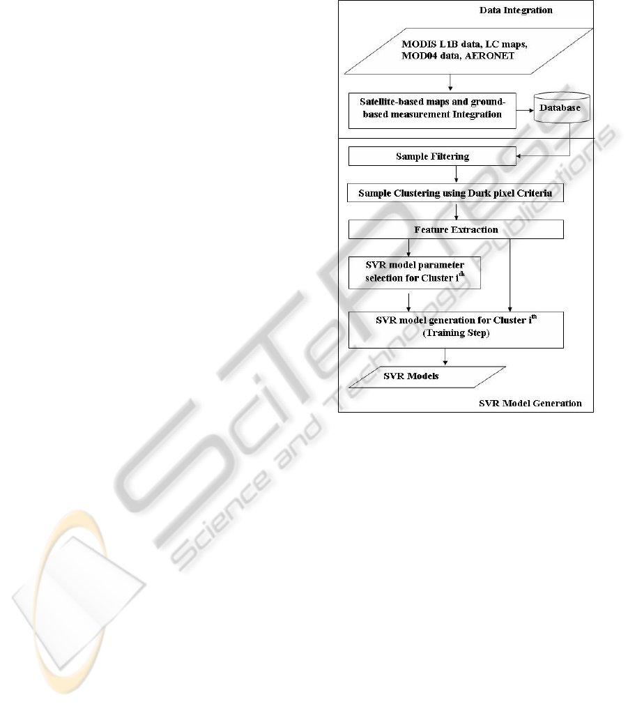
2 METHODOLOGIES

In this section, we present the methodologies to create

SVR models and to predict AOT maps from MODIS

data. Firstly, satellite-based data and ground-based

measurements in the areas of interest are collected.

Secondly, data from difference sources are integrated

to solve the differences of temporal and spatial reso-

lution. After that, ﬁltering and clustering techniques

exploiting physical aspects of data are applied in order

to reduce noise and total amount of data, and to sepa-

rate them into groups having different characteristics.

In the fourth step, SVR is used to create data model

for each cluster of data. The ﬂowchart of model gen-

eration is presented in Figure 1. Finally, in the map

prediction framework, aerosol maps at spatial resolu-

tion of 1 km

are derived from MODIS Level 1B data

using SVR models.

2.1 Data Collection

In this section, we describe the datasets used to de-

velop empirical data models as well as to input for

the map prediction framework. We collected the data

covering Europe in three years from 2007 to 2009 and

consisting of MODIS L1B data, MOD04 L2, Land

Cover (LC) map, and AERONET data Level 2.0.

MODIS L1B data acquired by MODIS sensors on

board the Terra and Aqua satellites present measure-

ments of a spectrum region from 0.415 to 14.235 µm

divided into 36 channels at 1 km, 500 m, and 250

m resolution at nadir. A scene covers an area on the

Earth surface of 2030 km in the direction of the satel-

lite orbit and of “1354 km” of non-uniform width (i.e.

the real pixel size projected on the earth far away

from nadir is larger than those at nadir because of

the inﬂuence of instrument scan and the earth’s cur-

vature) (Ren et al., 2010). The spectral reﬂectance

are calibrated, geo-located and provided in products

named MOD02 for Terra. In addition, the correspond-

ing geo-location product containing geodetic coordi-

nates, ground elevation, solar and satellite zenith and

azimuth angles for each 1 km sample is provided to-

gether with L1B data, known as MOD03 for Terra.

Figure 1: SVR approach for the AOT inversion problem.

MOD04 L2 is the aerosol products derived by

MODIS software package called Collection 005.

MOD04 L2 characterized by spatial resolution of

10x10 km

provide AOT estimations at seven wave-

lengths (0.470, 0.550, 0.670, 0.870, 1.240, 1.630

and 2.130 µm) over ocean and three wavelengths

over continental areas (0.470, 0.550 and 0.670 µm)

together with respective geometry information and

other various parameters. MOD04 L2 is used in val-

idation of SVR technique in both pixel and map do-

mains.

Land Cover maps present information of the Earth

surface which is used as an attribute contributed to

data modeling and as a mask for the cloud screening

process before applying aerosol retrieval algorithms.

LC maps are produced by a spectral rule-based soft-

ware system (MEEO, 2011) that provides 57 different

classes, out of which 40 refer to different land types.

AERONET is the global system of ground-

based Remote Sensing aerosol network established by

NASA and PHOTONS (University of Lille 1, CNES,

ICPRAM 2012 - International Conference on Pattern Recognition Applications and Methods

232

and CNRS-INSU) (NASA, 2011). Aerosol Optical

Thickness is measured by CIMEL Electronique 318A

spectral radiometers, sun and sky scanning sun pho-

tometers in various wavelengths: 0.340, 0.380, 0.440,

0.500, 0.670, 0.870, 0.940, and 1.020 µm, in intervals

of 15 minutes in average. After data processing steps,

cloud-screened and quality-assured data are stored

and provided as Level 2.0. In our work, AERONET

data Level 2.0 are collocated in space and synchro-

nized in time with satellite-based data, and then con-

sidered as target values for SVR models.

2.2 Data Integration

As described in the previous section, data are col-

lected from different sources have different temporal

and spatial resolutions which can be solved by the in-

tegration process. Satellite data include MODIS L1B

data (MOD02 and MOD03) and LC maps at 1 km

resolution, MODIS aerosol products (MOD04 L2) at

10 km

resolution. Ground-based data are obtained

from AERONET distributed sites.

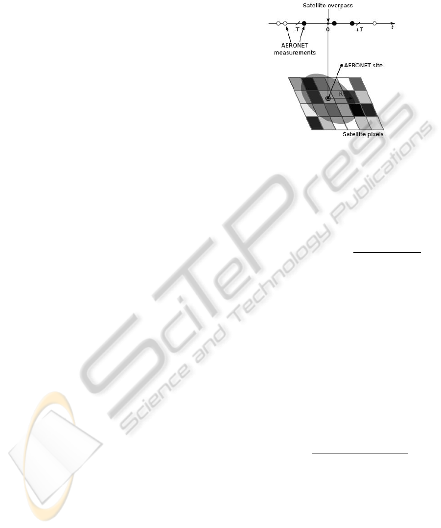
All satellite maps are acquired at the same time

and location, thus, only re-sampling process is ap-

plied to reﬁne MOD04 L2 products to 1 km

spa-

tial resolution. However, satellite-based and ground-

based data have different temporal resolution (every

day versus every 15 minutes, respectively) and dif-

ferent spatial resolution (1354 by 2030 of 1-km-pixel

maps in comparison with site points). Therefore,

we apply the time and location constrains to make

data integration, as proposed in (Ichoku et al., 2002).

Satellite data are considered if pixels are located over

land, cloudy-free and their distances from AERONET

sites are within radius R of 30 km. Meanwhile, the

contemporaneous measurements of AERONET in-

struments are selected and averaged within a tempo-

ral window T of 30 minutes around the satellite over-

passes. The integration is illustrated in Figure 2.

Satellite-based and ground-based integration is

applied to create data samples for data modeling

process. The usage of integrated data aims at im-

proving the aerosol retrieval quality by utilizing the

high accuracy of ground measurements as validated

in (Xu et al., 2005)(Vucetic et al., 2008)(Lary et al.,

2009)(Obradovic et al., 2010)(Nguyen et al., 2010b).

A sample is a combination of a satellite pixel’s at-

tributes and an arithmetic mean of AERONET AOT

values that satisﬁed collocation and time synchro-

nization constrains. A samples features consist of

the AERONET AOT at 0.553 µm, latitude, longi-

tude, sensor zenith angle, solar zenith angle, relative

azimuth angle, scattering angle, four reﬂectances at

0.646. 0.466, 1.243, and 2.119 µm, and land cover

class. The feature selection is replied on inputs of

LUT in the MODIS algorithm.

Figure 2: Spatio-temporal window for extracting satellite-

and ground-based measurements.

AERONET AOT at 0.553 µm (AOT

553

) is not

measured directly from AERONET sites and it is cal-

culated using log-linear interpolation from two AOT

values of the closest channels 0.500 and 0.670 µm (

AOT

500

and AOT

670

, respectively), as follows:

AOT

553

= e

log(AOT

500

)+(553−500)

log(AOT

670

)−log(AOT

500

)

670−500

(1)

The scattering angle Θ was deﬁned as:

Θ = cos

−1

(−cosθ

cosθ + sinθ

sinθcos φ) (2)

where θ

, θ and φ are the solar zenith, sensor view

zenith and relative azimuth angles, respectively.

2.3 Filtering and Clustering Techniques

The proposed ﬁltering and clustering techniques are

based on physical aspects of aerosol and satellite

measurements. The Top Of Atmosphere (TOA) re-

ﬂectance ρ

∗

at a particular wavelength λ , measured

by a satellite, can be approximated by

∗

= ρ

(θ

, θ, φ) +

dλ

(θ

(θ)ρ

(θ

, θ, φ)

1 − s

(θ

, θ, φ)

(3)

where ρ

is the atmospheric “path reﬂectance”, F

dλ

the “normalized downward ﬂux” for zero surface re-

ﬂectance, T

is the “upward total transmission” into

the satellite ﬁeld of view, s

is the “atmospheric

backscattering ratio” and ρ

is the angular “surface

reﬂectance”. They are functions of solar zenith an-

gle, satellite zenith angle, and solar/satellite relative

azimuth angles (θ

, θ and φ, respectively).

The equation (3) presents that a satellite mea-

sured reﬂectance is mainly contributed from aerosol

DOWNSCALING AEROSOL OPTICAL THICKNESS TO 1 KM2 SPATIAL RESOLUTION USING SUPPORT

VECTOR REGRESSION REPLIED ON DOMAIN KNOWLEDGE

233

reﬂectance (i.e. path reﬂectance ρ

) and surface re-

ﬂectance (i.e. ρ

). The functions F

dλ

, T

and s

also

depend on aerosol optical thickness though for small

surface reﬂectance they are less important. In phys-

ical algorithm, the path reﬂectance is separated and

used to derive aerosol optical thickness using built-

in parameters stored in LUT. The contribution of ρ

∗

from path reﬂectance is larger on short wavelengths

and low values of surface reﬂectance. Therefore, the

error for deriving AOT from this approximation is

smaller for dark surfaces. Dark pixels are determinate

by the mid-infrared channels (2.1 or 3.8 µm) because

those wavelengths are not effect by aerosol in the at-

mosphere.

Related to the ﬁltering technique applied on in-

tegrated datasets, we made an assumption that dark

pixels values are conﬁdent to select and match with

AERONET measurements. Then, integrated data are

grouped by acquisition time and AERONET location,

referred to as a combination set. In each combina-

tion set, samples are sorted on the mid infrared band

2.13 µm and then, 50% of brightest and 20% of dark-

est pixels are discarded. This ﬁltering process aims at

removing noisy data and chooses pixels towards dark-

ness for SVR model generation.

The proposed cluster technique is replied on pri-

ority of criteria applied over land surfaces exclud-

ing water, clouds, ice and snow to choose pixels for

aerosol derivation in the physical approach (Kaufman

and Tanre, 1997). The priorities are deﬁned as fol-

lows:

ﬁrst priority for 0.01 6 ρ

∗

2.1

6 0.05

second priority for ρ

∗

3.8

6 0.025

third priority for 0.01 6 ρ

∗

2.1

6 0.10

fouth priority for 0.01 6 ρ

∗

2.1

6 0.15

(4)

where ρ

∗

2.1

and ρ

∗

3.8

are TOA reﬂectance at wavelength

2.1 and 3.8 µm. The quality of the derivation is ex-

pected to decrease with the priority rank.

We proposed the clustering technique based on the

ﬁrst, third, and fourth priorities. Samples are sepa-

rated into four groups based on thresholds in the mid-

IR band 2.13 µm (from 0.01 to 0.05, from 0.05 to

0.10, from 0.10 to 0.15, and larger than 0.15). It aims

at specializing SVR models for particular data groups.

2.4 Support Vector Regression for

Inversion Process

SVR is applied for each cluster to create a correspond-

ing data model. This takes advantages of the divide-

and-conquer strategy and therefore, it is easier to con-

trol, improve, and evaluate the SVR performance on

each cluster.

The inversion problem is stated as follows. Given

a training dataset including l samples:

{(x

, y

), . . . , (x

, y

)} ⊂ X × ℜ (5)

where X denotes the space of the input patterns (i.e.

X ⊂ ℜ

), the target y

refers to as AERONET AOT

at 0.553 µm. The input is expressed as a record of

latitude, longitude, sensor zenith angle, solar zenith

angle, relative azimuth angle, scattering angle, re-

ﬂectance at 0.646 µm, reﬂectance at 0.466 µm, re-

ﬂectance at 1.243 µm, reﬂectance at 2.119 µm, and

land cover class. The ε-SVR, ﬁrstly introduced by

(Vapnik, 1995), is to ﬁnd the optimal function f (x)

that has at most ε deviation from the actually obtained

target y

from the training data. The ε-SVR with ep-

silon loss function and Radial Basic Function (RBF)

kernel provided by LIBSVM (Chang and Lin, 2011)

is used in our method.

The SVR algorithm is well known by generation

performance which can be achieved by good settings

of the ε-SVR parameters (i.e. regularization C, ε of

the lost function, and p in the kernel function RBF).

Because of high cost in cross validation for param-

eter selection on large datasets, we estimated those

parameters using a practical approach proposed in

(Cherkassky and Ma, 2004).

Following this method, the parameter C can be

chosen equal to the range of output y

values of train-

ing data. In order to limit the sensitiveness of C to

possible outliers in the training data, C is proposed as

C = max(| ¯y + 3σ

|, | ¯y − 3σ

|) (6)

where ¯y and σ are the mean and the standard deviation

of the y values of training data.

Parameter ε is estimated using the assumption that

the value of ε should be proportional to the input noise

variance. Based on the empirical results, the practical

ε is proposed as:

ε = tσ

lnl

(7)

where t, l and σ are the empirical dependency on the

number of training data (proposed as 3), the number

of samples in training data and the variance of addi-

tive noise δ, respectively. δ is described by:

y = f (x) + δ (8)

where δ is independent and identically distributed

(i.i.d) zero mean random noise, x is a multivariate in-

put and y is scalar output, f (x) is regression function.

We denotes

σ as the practical noise variance esti-

mated from training data which will be used as σ in

(7) for ε selection:

ICPRAM 2012 - International Conference on Pattern Recognition Applications and Methods

234

σ =

k − 1

∑

i=1

− ¯y

)

(9)

where k is window size, proposed in the 2 - 6 range, of

k-nearest-neighbours regression, ¯y

is a local average

of training data estimated from k nearest neighbours.

The width parameter p in RBF kernel is presented

as follows:

K(x

, x

) = e

−

−x

(10)

where x

is a training data.

p is appropriately selected to reﬂect the input range

of the training/test data. For the multivariate d-

dimensional problem, p is proposed to calculate as

∼ (0.1 − 0.5) where d input variables are pre-

scaled to [0, 1] range.

The parameter selection in our approach is carried

out on three steps:

• Initializing values of C, ε and p from training data

using the methodology described above.

• Tuning parameter ε by changing empirical de-

pendency parameter t in (7) to 30 (proposed as

3). It is due to our large training dataset, very

small target values, and repeated target values on

many samples as a result of integration process

in which many satellite pixels are matched to one

AERONET sites. Those lead to very small val-

ues of ε. The changing reduced number of sup-

port vectors to approximately 40% - 50% of total

number of training data and did not make strong

effect on Mean Square Error (MSE) received in

the cross-validation process.

• Tuning p in order to avoid the over-ﬁtting

when data models built on scatter data around

AERONET site are applied in map domain. This

step is based on two assumptions: (i) the ﬁne

aerosol prediction at 1 km

is not more accurate

than the coarse aerosol prediction at 10 km

be-

cause of data noise, and (ii) the prediction errors

increase by cluster priorities as mention in Sec-

tion 3.2. In implementation, we calculate MSE

of satellite MODIS AOT values and AERONET

data in the current working dataset. The MSE for

SVR models are selected from the range of clus-

ter 1 and cluster 2 whose pixels are considered

to be good for AOT derivation (i.e. from 0.060

to 0.075) for tuning p . The MSE on cluster 3

and 4 are large (∼ 0.1) and then are skipped be-

cause they lead to low accuracy of SVR model to

ground-truth AERONET values.

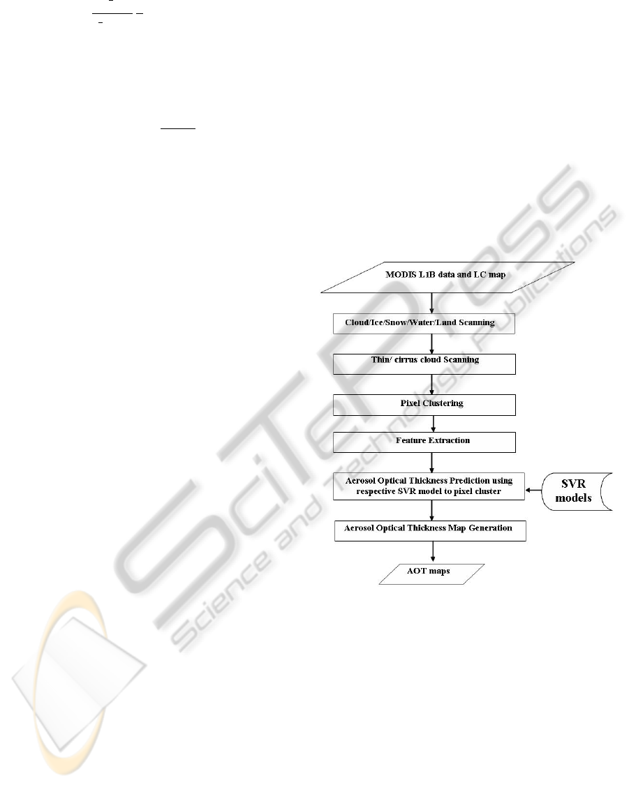
2.5 Map Prediction Framework

In this section, we introduce the map prediction

framework to derive AOT maps from MODIS L1B

data using generated SVR models. The ﬂowchart is

presented in Figure 3. The LC maps, produced by

SOIL MAPPER (MEEO, 2011), distinguish types of

pixels and perform the ﬁrst cloud screening. This is

due to the fact that aerosol estimation algorithm over

land is applied on pixels of land instead of cloud,

water, ice, snow. Because the AOT estimation on

cloud contamination or bright pixels from satellite re-

ﬂectance is not correct, we apply the second cloud

screening process using the cloud masking proce-

dure developed for retrieval of aerosol properties by

MODIS (Remer et al., 2004).

Figure 3: The map prediction framework.

The second cloud screening algorithm is based on

spatial variability of reﬂectances on TOA in the vis-

ible wavelengths. Clouds show the high spatial vari-

ability in the range from hundred meters to few kilo-

meters, while aerosol in general is very homogeneous.

The original algorithm is proposed in (Martins et al.,

2009) for cloud masking over ocean but this proce-

dure has been extended to land and applied in both

aerosol algorithms in Collection 005. The land algo-

rithm generates a cloud mask using spatial variabil-

ity of the 0.47 and 1.38 µm channels with thresholds

0.0025 and 0.003, respectively. If the standard devia-

tion calculated for each group of 3 x 3 pixels is greater

than the corresponding threshold, then the area of the

entire 3 x 3 pixel box is considered as clouds. In

DOWNSCALING AEROSOL OPTICAL THICKNESS TO 1 KM2 SPATIAL RESOLUTION USING SUPPORT

VECTOR REGRESSION REPLIED ON DOMAIN KNOWLEDGE

235

addition, tests on visible channel reﬂectance thresh-

olds are carried out. If the reﬂectance at 0.47 µm and

1.38 µm are greater than 0.4 and 0.025, respectively,

the pixel is considered as a cloudy pixel. In our ap-

proach, all calculations are applied at 1 km

resolu-

tion for both 0.47 µm and 1.38 µm channels instead

of 500 m and 1 km

resolutions, respectively as in the

Collection 5 algorithm.

After cloud scanning processes, selected pixels

are grouped into four clusters in order to apply the

corresponding SVR data model to predict aerosol op-

tical thickness. The ﬁnal process collects predicted

pixels, integrates with geo-information and then gen-

erates the AOT map.

3 EXPERIMENTS AND RESULTS

3.1 Pixel Domain

In this section, we present experiments on pixel do-

main referred to as pixels collected in areas around

AERONET sites and used to make and test SVR mod-

els.

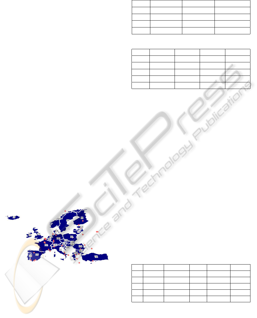
The data, covering Europe in three year from 2007

to 2009, consist of MODIS L1B data and LC map

at 1 km

resolution, MOD04 L2 at 10 km

resolu-

tion, and AERONET data Level 2.0. After integrating

satellite-based and ground-based measurements, we

obtained data, called samples afterward, at 35, 42 and

36 AERONET sites for 2007, 2008, and 2009, respec-

tively. The sites distribution is presented in Figure 4.

Figure 4: Distribution of AERONET sites over the Europe

area used in data modeling.

The statistics on total dataset before and after ap-

plication of ﬁlter is presented in detail in Table 1. 30%

out of the total 3,570,245 samples is remained after

ﬁltering. In the next step, those samples are grouped

into four groups based on proposed thresholds of the

mid-infrared band 2.13 µm as described in the Section

2.3. As shown in Table 2, cluster 1, 2 and 3, consid-

ered as having good pixels for AOT estimation, hold

most of data, i.e. 22.53%, 55.94% and 16.98% of to-

tal, respectively.

Table 1: Statistics on total dataset.

Year # AER site # Raw data Filtered data

2007 35 1,331,210 402,871

2008 42 1,242,157 376,323

2009 36 996,878 301,981

# 3,570,245 1,081,175

Table 2: Statistics on different clusters.

Year # Clus.1 # Clus.2 # Clus.3 # Clus.4

2007 86,593 223,625 72,479 20,136

2008 95,875 207,968 60,822 11,584

2009 61,167 173,261 50,299 17,169

# 243,635 604,854 183,600 48,889

% 22.53% 55.94% 16.98% 4.52%

For each cluster, 10,000 random samples are se-

lected for each year to create training datasets, while

the left data are used as testing datasets. The evalua-

tion was carried out on each cluster using Mean Error

(ME), Root Mean Square Error (RMSE) and COR-

relation coefﬁcient (COR) all of which are calculated

from AOT values obtained by different methods.

Table 3 shows the accuracy of SVR predictors

in comparison with AERONET measurements on the

pixel domain. In this experiment, all estimated AOT

values using SVR are matched directly to correspond-

ing AERONET values and validated. Using the pro-

posed approach, four clusters achieve acceptable ac-

curacy (COR ∼ 0.78 and RMSE ∼ 0.070). How-

ever, SVR models slightly underestimate AOT values,

represented by negative ME. The general results on

COR, RMSE, and ME, calculated by proportion of

quantity of pixels in each cluster to the total number

of pixels, are 0.782, 0.0694, and -0.0495, respectively.

These results are considered as acceptable for AOT

estimation at 1 km

of resolution where inputs are

very variant and noisy in comparison with data used

in coarser spatial resolution application (e.g. 10x10

of MODIS AOT).

Table 3: SVR prediction on different clusters.

C. # SV # Testing COR RMSE ME

1 12,131 213,635 .795 .061150 -.0045

2 13,012 574,854 .780 .069747 -.0048

3 15,451 153,600 .775 .078532 -.0056

4 16,506 18,889 .774 .077550 -.0080

# 960,978 .782 .069393 -.0049

Another experiment is carried out on three pairs

of AOT, that is, SVR AOT and AERONET AOT

(SVR - AER), MOD04 L2 AOT and AERONET AOT

(MODIS - AER), SVR AOT and MOD04 L2 AOT

(SVR - MODIS). As described in Section 2.4, we cre-

ated SVR models with MSE of SVR predicted values

and AERONET target bounded by MSE of MODIS

ICPRAM 2012 - International Conference on Pattern Recognition Applications and Methods

236

AOT and AERONET AOT in order to avoid over-

ﬁtting. Therefore, the SVRs will have similar perfor-

mance as MODIS algorithm on good pixels (clusters

1 and 2) in theory. This experiment aims at investigat-

ing the relationship between SVR AOT and MODIS

AOT around AERONET site to explain the results of

the next validation in which we predict and compare

directly AOTs on map domain.

In the second experiment, all SVR AOT and

MODIS AOT are aggregated by acquisition time and

AERONET site, then averaged and validated to cor-

responding AERONET values. This method will give

more stable validation results when data at different

spatial resolutions are compared.

Table 4 presents the obtained results. Firstly,

the assumption about prediction quality decreased by

cluster, as mentioned in Section 2.3, is presented cor-

rectly in this experiment. For both SVR and MODIS

algorithm, the correlation of AOT values (COR)

decreases while errors (RMSE) increases gradually

from cluster 1 to cluster 4.

Table 4: Comparison among aggregated SVR AOT, aggre-

gated MODIS AOT and AERONET AOT for cluster 1, 2, 3,

4 (top to bottom).

# SVR - AER MODIS - AER SVR - MODIS

COR RMSE COR RMSE COR RMSE

2317 .778 .0633 .802 .0641 .858 .0575

4555 .809 .0722 .825 .0757 .841 .0763

1968 .791 .0776 .765 .1003 .728 .1065

547 .694 .0785 .626 .1041 .375 .1186

The prediction errors are similar to MODIS AOT

and SVT AOT on cluster 1 and 2 (RMSE ∼ 0.064

and 0.072, respectively). However, SVR AOT are

more accurate than MODIS AOT on clusters 3 and

4 (RMSE = 0.077 and 0.078 vs. 0.100 and 0.104).

As the result, SVR AOT and MODIS AOT are com-

parable on cluster 1 and 2 (COR ∼ 0.858 and 0.841,

RMSE ∼ 0.057 and 0.076, respectively) but large dif-

ferent on clusters 3 and 4 (COR ∼ 0.728 and 0.375,

RMSE ∼ 0.106 and 0.118, respectively). The corre-

lation between SVR AOT and MODIS AOT is pre-

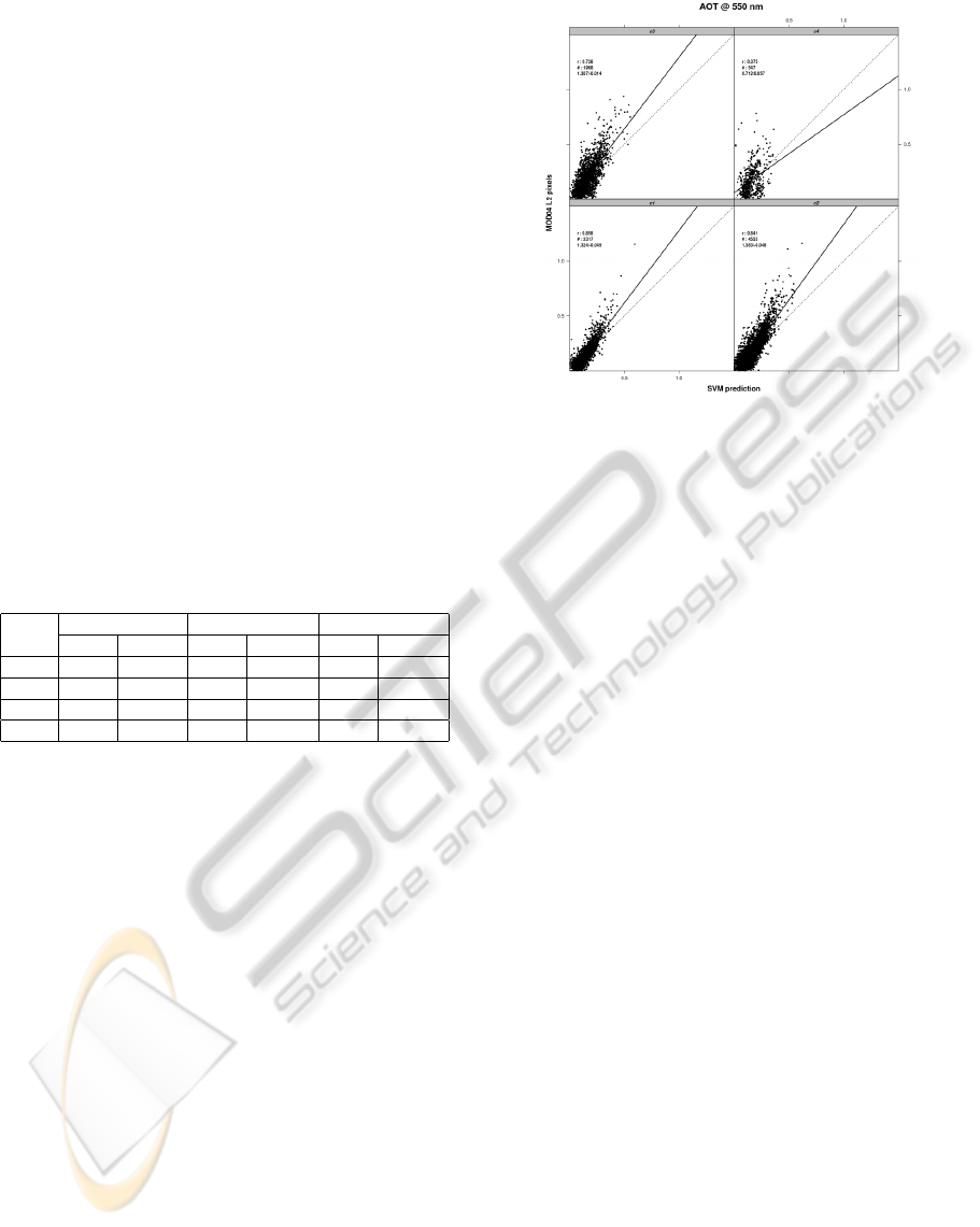
sented in the aggregated AOT scatter plot in Figure 5.

The relationship is worst on the cluster 4.

3.2 Map Domain

Map domain refers to all cloud-free pixels on im-

ages recorded by MODIS. The experiment carried out

in map domain aims at evaluating quality of SVR

models when they are used to derived AOT map

from MODIS L1B data. The validation of algorithms

working on map domain, up to now, is still a chal-

lenging problem because there are no conﬁdent tar-

get values for comparison. MOD04 L2 maps, con-

Figure 5: The scatter plot between SVR AOT and MODIS

AOT for cluster 1, 2, 4 and 3 (right-left, bottom-top order).

sidered as one of the best products for aerosol mon-

itoring at global scale nowadays, are used in our ex-

periment. However, as shown in the previous section,

re-sampled MODIS AOT also presents low quality in

comparison with ground truth AERONET AOT for

some certain cases (e.g. pixels of cluster 4).

We collected one map per month in three years

from 2007 to 2009 covering the area of Italy as il-

lustrated in Figure 6. Thus, the validation dataset

consists of 36 images. After applying the map pre-

diction framework, as presented in the section 2, we

received 36 AOT maps at 1 km

spatial resolution.

Corresponding MOD04 L2 maps are collected and

re-sampled into 1 km

maps by simply dividing one

10x10 km

pixel to one hundred of 1x1 km

pixels

with same AOT values. Since the algorithms work on

different spatial resolutions and use different method-

ologies for scanning good pixels, the two AOT maps

are not completely overlapped. Therefore, the COR

and RMSE are calculated only on match pixels which

have both SVR AOT and MODIS AOT. An illustra-

tion of AOT map estimated by our SVR and MODIS

algorithm is shown in Figure 7.

Table 5 presents the numerical results of the ex-

periment on validation datasets. SVR AOT of clus-

ters 1 and 2, occupying a big quantity of data (41.72%

and 44.74%, respectively), have small errors and good

correlation in comparison with MODIS AOT (COR

∼ 0.78, RMSE ∼ 0.057). The worst case hap-

pens to cluster 4 with COR = 0.401 and RMSE =

0.1213. Regarding the validation between SVR AOT

and MODIS AOT in pixel domain, obtained results

are generally consistent. In details, the decrease of

COR can be observed in clusters 1, 2, and 3 while

RMSE is slightly increase, especially on cluster 3.

DOWNSCALING AEROSOL OPTICAL THICKNESS TO 1 KM2 SPATIAL RESOLUTION USING SUPPORT

VECTOR REGRESSION REPLIED ON DOMAIN KNOWLEDGE

237

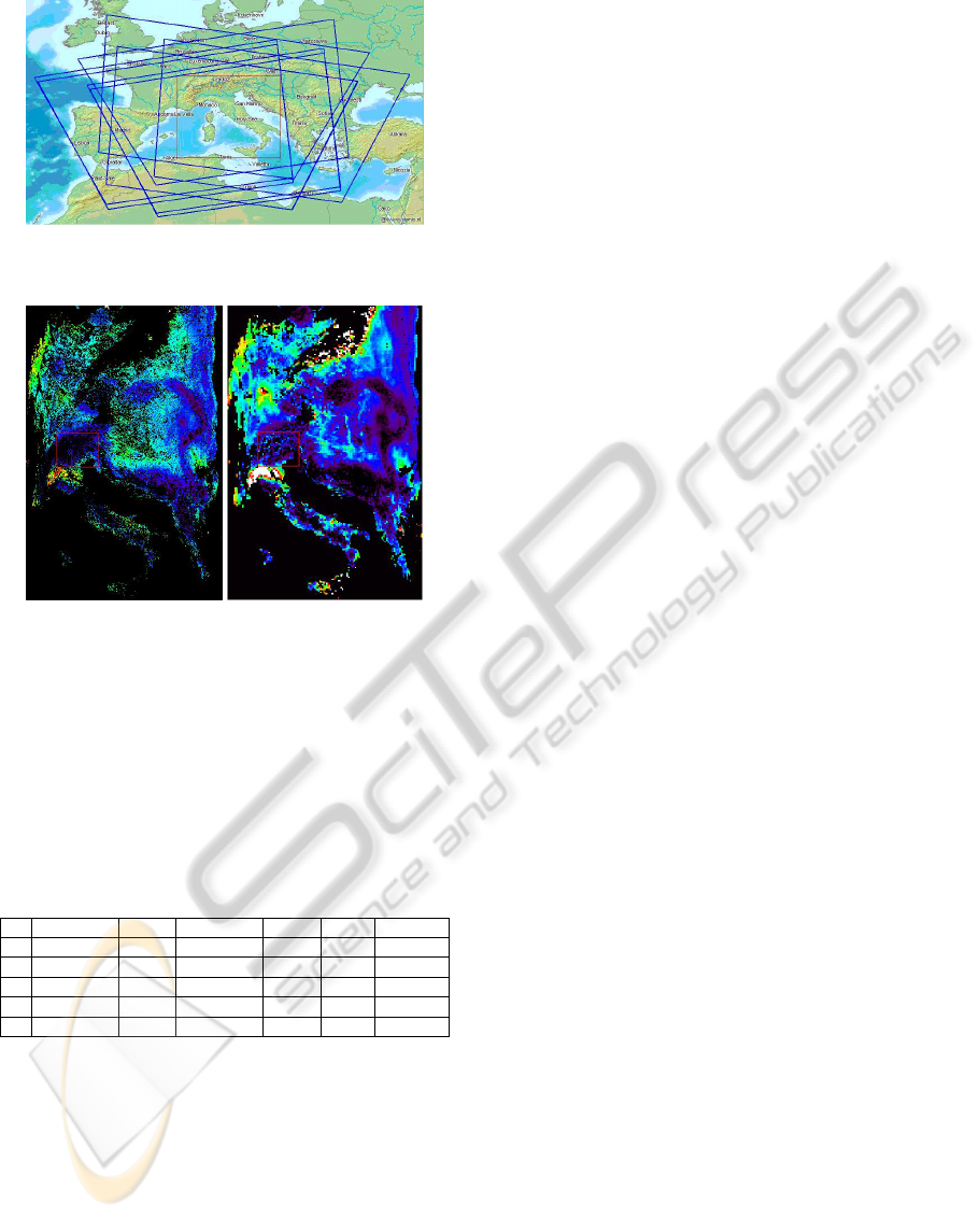
Figure 6: Illustration of MODIS L1B maps covering our

area of interest (the red square) in June 2008.

Figure 7: SVR AOT map (left) and re-sample MODIS AOT

map (right) for the dataset 20072660955005.

The difference of validation dataset and aggregation

and instance comparison can be explained for this sit-

uation. The general COR and RSME are moderate

and acceptable (0.769 and 0.0613, respectively).

Table 5: SVR MODIS validation for different clusters on

the map domain (C: cluster, #T: total number of pixels,

%T: percentage of cluster pixels on total, #N: number of

matched pixels, %N: percentage of matches on total num-

ber of cluster)

C #T %T #M %M COR RMSE

1 3,003,802 41.72 2,393,443 83.71 .782 .053846

2 3,221,464 44.74 3,070,472 91.62 .792 .061518

3 712,496 9.89 685,974 80.15 .684 .075537

4 262,812 3.65 126,675 46.64 .401 .121253

7,200,574 6,276,564 75.28 .769 .061330

The map domain validation results are various for

different datasets but following conclusions can be in-

ferred. Firstly, the scanning of good pixels in our map

prediction framework sweeps out many pixels of the

cluster 3 and 4 because strictly constrains are applied,

which is shown by a smaller amount of their pixels

in compare with cluster 1 and 2. However, this pro-

cess is necessary when estimation is carried out di-

rectly on values of 1 km

pixel in stead of averaged

values of good pixels at 500 m selected in a box sized

10x10 km

as in MODIS algorithm. Secondly, the

proposed SVR methodology performs well on most

pixels of cluster 1 and 2, presented by good COR and

low RMSE. Finally, the algorithm seems not work sta-

bly on pixels of the cluster 3. Some datasets have low

COR in comparison with MODIS AOT. Also, the bad

results are observed in pixels of the cluster 4. In fact,

SVR models are built on AERONET AOT targets. As

shown in the previous experiments, the relationship

between SVR AOT and MODIS AOT is not really

good for the cluster 3 and worse for cluster 4 in the

pixel domain. More investigation on pixels of cluster

3 and 4 should be done in both physical and inversion

algorithm aspects.

4 CONCLUSIONS

In this article, we proposed the methodology to esti-

mate aerosol optical thickness at 1 km

from MODIS

L1B data using SVR relied on domain knowledge. In

the proposed approach, the satellite-based data and

ground-based measurements over areas of interest are

collected and integrated using temporal and spatial

constrains. After that, ﬁltering and clustering tech-

niques are applied in order to reduce noise and total

amount of data, and to separate them into four groups

having different characteristics. Then, SVR technique

is applied to create corresponding data models. Fi-

nally, in the prediction framework, aerosol maps at

spatial resolution of 1 km

is derived from MODIS

L1B data using SVR models retrieved in the previous

step.

Experiments were carried out on data from 2007

to 2009, covering European areas, in both pixel and

map domain. The evaluation results show that the

proposed approach deals well with two mentioned ar-

guments: (i) a very large and noisy dataset and (ii)

the movement from pixel domain to map domain,

presented as good quality of SVR AOT at 1 km

resolution in comparison with values measured by

AERONET and MODIS algorithm. Advantages of

the usage of the cluster technique are proved when

speciﬁc SVR models are created for different groups

of data. Thus, the modeling of large and variant

dataset is controllable and more effective. As a result,

good and bad aerosol predictors using SVR models

are pointed out, and therefore, investigation and im-

provement will be done further.

In future, we will focus on estimation of AOT in

map domain. The inversion algorithms for spatial

data will be investigated more deeply. Also, the val-

idation will be extended on other areas. Application

of the proposed methodology on data recorded by dif-

ferent satellite sensors will be aimed at.

ICPRAM 2012 - International Conference on Pattern Recognition Applications and Methods

238

REFERENCES

Chang, C. and Lin, C. (2011). LIBSVM: A Library for

Support Vector Machines.

Chen, Q. and Shao, Y. (2008). The Application of Im-

proved BP Neural Network Algorithm in Urban Air

Quality Prediction: Evidence from China. In Proceed-

ing of 2008 IEEE Paciﬁc-Asia Workshop on Computa-

tional Intelligence and Industrial Application (PACIIA

2008), pages 160–163.

Cherkassky, V. and Ma, Y. (2004). Practical Selection of

SVM Parameters and Noise Estimation for SVM Re-

gression. In Neural Networks, volume 17, pages 113–

126.

Han, B., Vucetic, S., Braverman, A., and Obradovic, Z.

(2006). A Statistical Complement to Deterministic Al-

gorithms for the Retrieval of Aerosol Optical Thick-

ness from Radiance Data. In Engineering Applica-

tions of Artiﬁcial Intelligence, volume 19, pages 787–

795. Pergamon Pess.

Ichoku, C., Chu, D., Mattoo, S., Kaufman, Y., Remer, L.,

Tanr, D., Slutsker, I., and Holben, B. (2002). A spatio-

temporal approach for global validation and analysis

of MODIS aerosol products. In Geophysical Research

Letter, volume 29, pages 1–4.

Kaufman, Y. J. and Tanre, D. (1997). Algorithm for re-

mote sensing of tropospheric aerosol from modis. In

MODIS ATBD. NASA.

Lary, D., Remer, L., MacNeill, D., Roscoe, B., and Par-

adise, S. (2009). Machine Learning Bias Correction of

MODIS Aerosol Optical Depth. In IEEE Geoscience

and Remote Sensing Letters, volume 4, pages 694–

698.

Li, C., Lau, A., Mao, J., and Chu, D. (2005). Retrieval,

Validation, and Application of the 1-km Aerosol Op-

tical Depth from MODIS Measurements over Hong

Kong. In IEEE Transactions on Geoscience and Re-

mote Sensing, volume 43, pages 2650–2658.

Lu, W., Wang, W., Leung, A., Lo, S., Yuen, R., Xu, Z., and

Fan, H. (2002). Air Pollutant Parameter Forecasting

Using Support Vector Machine. In Proceeding of the

2002 International Joint Conference on Neural Net-

work (IJCNN02), pages 630–635.

Martins, J., Tanr, D., Remer, L., Kaufman, Y., Matto, S.,

and Levy, R. (2009). MODIS cloud screening for

remote sensing of aerosols over oceans using spa-

tial variability. In Geophysical Research Letters, vol-

ume 29.

MEEO, M. E. E. O. (2011). SOIL MAPPER

.

NASA (2011). AErosol Robotic Network (AERONET).

Nguyen, T., Mantovani, S., and Bottoni, M. (2010a). Es-

timation of Aerosol and Air Quality Fields with PM

MAPPER An Optical Multispectral Data Processing

Package. In ISPRS TC VII Symposium 100 year IS-

PRS, volume XXXVIII(7A), pages 257–261.

Nguyen, T., Mantovani, S., Campalani, P., Cavicchi, M.,

and Bottoni, M. (2010b). Aerosol Optical Thickness

Retrieval from Satellite Observation Using Support

Vector Regression. In Progress in Pattern Recogni-

tion, Image Analysis, Computer Vision, and Appli-

cations - 15th Iberoamerican Congress on Pattern

Recognition (CIARP2010), pages 492–499. Springer.

Obradovic, S., Das, D., Radosavljevic, V., Ristovski, K.,

and Vucetic, S. (2010). Spatio-Temporal Characteri-

zation of Aerosols through Active Use of Data from

Multiple Sensors. In ISPRS TC VII Symposium 100

year ISPRS, volume XXXVIII(7B), pages 424–429.

Okada, Y., Mukai, S., and Sano, I. (2001). Neural Network

Approach for Aerosol Retrieval. In IEEE 2001 Inter-

national Geoscience and Remote Sensing Symposium

(IGARSS01), volume 4, pages 1716–1718.

Oo, M., Hernandez, E., Jerg, M., Moshary, B., and Ahmed,

S. (2008). Improved MODIS Aerosol Retrieval Using

Modiﬁed VIS/MIR Surface Albedo Ratio over Urban

Scenes. In IEEE 2008 International Geoscience and

Remote Sensing Symposium (IGARSS08), volume 3,

pages 977–979.

Osowski, S. and Garanty, K. (2006). Wavelets and Sup-

port Vector Machine for Forecasting the Meteorologi-

cal Pollution. In Proceeding of the 7th Nordic Signal

Processing Symposium (NORSIG), pages 158–61.

Ramakrishnan, R., Schauer, J., Chen, L., Huang, Z., Shafer,

M., Gross, D., and Musicant, D. (2005). The EDAM

project: Mining atmospheric aerosol datasets. In In-

ternational Journal of Intelligent Systems, volume 20

(7), pages 759–787.

Remer, L., Tanr, D., and Kaufman, Y. (2004). Algorithm

for Remote Sensing of Tropospheric Aerosol from

MODIS: Collection 5. In MODIS ATBD. NASA.

Ren, R., Guo, S., and Gu, L. (2010). Fast bowtie effect

elimination for MODIS L1B data. In The Journal of

China Universities of Posts and Telecommunications,

volume 17(1), pages 120–126. Elsevier.

Siwek, K., Osowski, S., Garanty, K., and Sowinski, M.

(2008). Ensemble of Neural Predictors for Forecast-

ing the Atmospheric Pollution. In IEEE International

Joint Conference on Neural Network, pages 643–648.

Vapnik, V. (1995). The nature of statistical learning theory.

Springer-Verlag, Berlin.

Vucetic, S., Han, B., Mi, W., Li, Z., and Obradovic, Z.

(2008). A Data-Mining Approach for the Validation

of Aerosol Retrievals. In IEEE Geoscience and Re-

mote Sensing Letter, volume 5(1), pages 113–117.

Xu, Q., Obradovic, Z., Han, B., Li, Y., Braverman, A., and

Vucetic, S. (2005). Improving Aerosol Retrieval Ac-

curacy by Integrating AERONET, MISR and MODIS

Data. In The 8th Intenational Conference on Informa-

tion Fusion, volume 1.

DOWNSCALING AEROSOL OPTICAL THICKNESS TO 1 KM2 SPATIAL RESOLUTION USING SUPPORT

VECTOR REGRESSION REPLIED ON DOMAIN KNOWLEDGE

239