
ON THE VC-DIMENSION OF UNIVARIATE DECISION TREES
Olcay Taner Yildiz
Department of Computer Engineering, Is¸ık University, 34980, S¸ile,
˙
Istanbul, Turkey
Keywords:
VC-Dimension, Decision trees.
Abstract:
In this paper, we give and prove lower bounds of the VC-dimension of the univariate decision tree hypothesis
class. The VC-dimension of the univariate decision tree depends on the VC-dimension values of its subtrees
and the number of inputs. In our previous work (Aslan et al., 2009), we proposed a search algorithm that
calculates the VC-dimension of univariate decision trees exhaustively. Using the experimental results of that
work, we show that our VC-dimension bounds are tight. To verify that the VC-dimension bounds are useful,
we also use them to get VC-generalization bounds for complexity control using SRM in decision trees, i.e.,
pruning. Our simulation results shows that SRM-pruning using the VC-dimension bounds finds trees that are
more accurate as those pruned using cross-validation.
1 INTRODUCTION
In pattern recognition the knowledge is extracted as
patterns from a training sample for future prediction.
Most pattern recognition algorithms such as neural
networks (Bishop, 1995) or support vector machines
(Vapnik, 1995) make accurate predictions but are not
interpretable, on the other hand decision trees are
simple and easily comprehensible. They are robust
to noisy data and can learn disjunctive expressions.
Whatever the learning algorithm is, the main goal of
the learner is to extract the optimal model (the model
with least generalization error) from a training set. In
the penalization approaches, the usual idea is to de-
fine the generalization error in terms of the training
error and the complexity of the model.
One problem in estimating the generalization error
is to specify the number of free parameters h when the
estimator is not linear. In the statistical learning the-
ory (Vapnik, 1995), Vapnik-Chervonenkis (VC) di-
mension is a measure of complexity defined for any
type of estimator. VC dimension for a class of func-
tions f(x,α) where α denotes the parameter vector
is defined to be the largest number of points that can
be shattered by members of f(x,α). A set of data
points is shattered by a class of functions f(x, α) if
for each possible class labeling of the points, one can
find a member of f(x,α) which perfectly separates
them. For example, the VC dimension of the linear
estimator class in d dimensions is d + 1 which is also
the number of free parameters.
Structural risk minimization (SRM) (Vapnik,
1995) uses the VC dimension of the estimators to se-
lect the best model by choosing the model with the
smallest upper bound for the generalization error. In
SRM, the possible models are ordered according to
their complexity
M
0
⊂ M
1
⊂ M
2
⊂ ... (1)
For example, if the problem is selecting the best de-
gree of a polynomial function, M
0
will be the polyno-
mial with degree 0, M
1
will be the polynomial with
degree 1, etc. For each model, the upper bound for its
generalization error is calculated. For binary classifi-
cation, the upper bound for the generalization error is
(Cherkassky and Mulier, 1998)
E
g
= E
t
+
ε
2
1+
r
1+
4E
t
ε
!
(2)
and ε is given by the formula
ε = a
1
V[log(a
2
N/V) + 1] −log(ν)
N
(3)
where V represents the VC dimension of the model, ν
represents the confidence level, and E
t
represents the
training error. It is recommended to use ν =
1
√
N
for
large sample sizes.
In this work, we use decision trees as our hypothe-
sis class. In a univariatedecision tree (Quinlan, 1993),
the decision at internal node m uses only one attribute,
i.e., one dimension of x, x
j
. If that attribute is discrete,
there will be L children (branches) of each internal
node corresponding to the L different outcomes of the
205
Taner Yildiz O. (2012).
ON THE VC-DIMENSION OF UNIVARIATE DECISION TREES.
In Proceedings of the 1st International Conference on Pattern Recognition Applications and Methods, pages 205-210
DOI: 10.5220/0003777202050210
Copyright
c
SciTePress

decision. ID3 is one of the best known univariate de-
cision tree algorithm with discrete features (Quinlan,
1986).
As far as our knowledge, there is no explicit for-
mula for the VC-dimension of a decision tree. Al-
though there are certain results for the VC-dimension
of decision trees such as (i) it is known that the VC
dimension of a binary decision tree with N nodes and
dimension d is between Ω(N) and O (N logd) (Man-
sour, 1997) (ii) it is shown that the VC dimension of
the set of all boolean functions on N boolean variables
defined by decision trees of rank at most r is
∑
r
i=0
n
i
(Simon, 1991), the bounds are structure independent,
that is, they give the same bound for all decision trees
of size N.
In this work, we first focus on the easiest case
of univariate trees with binary features and we prove
that the VC-dimension of a univariate decision tree
with binary features depends on the number of bi-
nary features and the tree structure. As a next step,
we generalize our work to the univariate decision tree
hypothesis class, where a decision node can have L
children depending on the number of values of the se-
lected feature. We show that the VC-dimension of
L-ary decision tree is greater than or equal to the VC-
dimension of its subtrees. Based on this result, we
give an algorithm to find a lower bound of the VC-
dimension of a L-ary decision tree. We use these VC-
dimension bounds in pruning to validate that they are
indeed tight bounds.
This paper is organized as follows: In Section
2, we give and prove the lower bounds of the VC-
dimension of the univariate decision trees with binary
features. We generalize our work to L-ary decision
trees in Section 3. We give experimental results in
Section 4 and conclude in Section 5.
2 VC-DIMENSION OF THE
UNIVARIATE DECISION TREES
WITH BINARY FEATURES
We consider the well-known supervised learning set-
ting where the decision tree algorithm uses a sample
of m labeled points S = ((x
(1)
,y
(1)
),...,(x
(m)
,y
(m)
) ∈
(X ×Y)
m
, where X is the input space and Y the label
set, which is {0,1}. The input space X is a vectorial
space of dimension d, the number of features, where
each feature can take values from {0,1}. From this
point on, we refer only internal nodes of the decision
tree as node(s).
Theorem 1. The VC-dimension of a single decision
node univariate decision tree that classifies d dimen-
x
(1)
x
(2)
x
(3)
x
(4)
x
1
1
0
0
0
x
2
0
1
0
0
x
3
0
0
1
0
x
4
0
0
0
1
x
5
1
1
0
0
x
6
1
0
1
0
x
7
1
0
0
1
x
5
0
1
x
(1)
x
(2)
x
(3)
x
(4)
x
3
0
1
x
(3)
x
(4)
x
(1)
x
(2)
(1)
(1)
(0)
(0)
(1)
(0)
(0)
(0)
Figure 1: Example for Theorem 1 with d = 7 and m = 4. If
the class labeling of S is {1, 1, 0, 0} we select feature 5 (left
decision tree). If the class labeling of S is {0, 0, 1, 0} we
select feature 3 (right decision tree).
sional data is ⌊log
2
(d + 1)⌋+ 1.
Proof. To show the VC-dimension of the single de-
cision node univariate decision tree is at least m, we
need to find such a sample S of size m that, for each
possible class labelings of these m points, there is an
instantiation h of our single node decision tree hy-
pothesis class H that classifies it correctly. We con-
struct the sample S such that each feature x
i
cor-
responds to a distinct possible class labeling of m
points, implying a one-to-one mapping between class
labelings and features (namely identity function since
both features and class labelings come from the same
set). So for each possible class labeling, we will
choose the decision tree hypothesis h which has the
corresponding feature as the split feature (See Figure
1 for an example). A sample with m examples can be
divided into two classes in 2
m−1
−1 different ways. If
we set the number of features to that number:
d = 2
m−1
−1
d + 1 = 2
m−1
log
2
(d + 1) = m−1
m = log
2
(d + 1) + 1
Theorem 2. The VC-dimension of a degenerate uni-
variate decision tree with N nodes that classifies d
dimensional data is at least ⌊log
2
(d −N + 2)⌋+ N.
ICPRAM 2012 - International Conference on Pattern Recognition Applications and Methods
206

x
(1)
x
(2)
x
(3)
x
(4)
x
1
1
0
0
0
x
2
0
1
0
0
x
3
1
1
0
0
x
4
0
0
0
1
x
5
0
0
0
0
x
6
0
0
0
0
x
7
0
0
0
0
x
7
0
1
x
(5)
x
(6)
x
(7)
0 0 0 0
1 0 0
0 0 0 0 0 1 0
0 0 0 0 0 0 1
x
(7)
x
6
0
1
x
(6)
x
5
0
1
x
(5)
x
4
0
1
x
(4)
x
3
0
1
x
(1)
(1)
x
(2)
(1)
x
(3)
(0)
Figure 2: Example for Theorem 2 with d = 7 and m = 7.
If the class labeling of S is {1, 1, 0, x, x, x, x} we select
feature 3 in the bottom node. The labelings of the last four
examples do not matter since they are alone in the leaves
they reside.
In a degenerate decision tree each node (except the
bottom one) has a single child node.
Proof. Similar to the Theorem 1, we produce a sam-
ple S such that, for each possible class labelings of
this sample, there is an instantiation h of our degener-
ate decision tree hypothesis class H that classifies the
sample correctly. We proceed in a bottom-up fash-
ion. The bottom node can classify m examples by
setting up 2
m−1
−1 features to produce a one-to-one
mapping between class labelings and those features
(See Theorem 1). We also add one feature and one
example for each remaining node, where the value of
the new feature is 1 for the corresponding example
and 0 for the remaining examples (See Figure 2 for
an example). The classification of the sample goes
as follows: N −1 nodes (which have a single child
node) will select the new N −1 features respectively
as the split features so that each added example will
be forwarded to the leaf of the corresponding node
alone. The remaining m examples will be forwarded
to the bottom node, where the decision node can clas-
sify those examples whatever their class combination
is. The number of features is,
d = 2
m−1
−1+ N−1
d −N + 2 = 2
m−1
m = log
2
(d −N + 2) + 1
So the VC-dimension of the degenerate decision tree
is at least (m + N −1), that is ⌊log
2
(d −N + 2)⌋+
N.
Theorem 3. The VC-dimension of a full univariate
decision tree of height h that classifies d dimensional
data is at least 2
h−1
(⌊log
2
(d −h + 2)⌋+ 1). In a full
decision tree each node has two child nodes.
x
(1)
x
(2)
x
(3)
x
1
1
0
0
x
2
0
1
0
x
3
1
1
0
x
4
0
0
0
x
5
0
0
0
x
5
0
1
x
(1)
x
(2)
x
(3)
(1)
(0)
(0)
x
(4)
x
(5)
x
(6)
1
0
0
0
1
0
1
1
0
0
0
0
1
1
1
x
(7)
x
(8)
x
(9)
1
0
0
0
1
0
1
1
0
1
1
1
0
0
0
x
(10)
x
(11)
x
(12)
1
0
0
0
1
0
1
1
0
1
1
1
1
1
1
x
4
0
1
x
4
0
1
x
1
0
1
x
2
0
1
x
2
0
1
x
3
0
1
x
(5)
x
(4)
x
(6)
(1)
(0)
(0)
x
(8)
x
(7)
x
(9)
(1)
(0)
(0)
x
(10)
x
(12)
x
(11)
(1)
(0)
(1)
Figure 3: Example for Theorem 3 with d = 5 and m = 12.
Using feature 5 in the first level and feature 4 in the second
level, one divides the class labelings into 4 subproblems of
m = 3. Each subproblem can then be shattered with a single
node.
Proof. Similar to the Theorem 2 we proceed in a bot-
tom up fashion. Each bottom node (For this case,
there are 2
h−1
of them) can classify m examples by
setting up 2
m−1
−1 features to produce a one-to-one
mapping between class labelings and those features
(See Theorem 1). We also add h −1 features to the
sample, where the first feature will be used in the first
level, the second feature will be used in the second
level, etc. (See Figure 3 for an example). This way
each bottom node can be labeled as a h −1 digit bi-
nary number, which corresponds to the values of the
new h −1 features of the examples forwarded to that
node. For example, the values of the first, second,
..., h−1’th features (added features) of the examples
forwarded to leftmost bottom node will be 0. On the
other hand, the values of the first, second, ..., h−1’th
features of examples forwarded to the rightmost bot-
tom node will be 1. Given such a setup, one can pro-
duce a full decision tree which can classify 2
h−1
m
points for each possible class labeling. The number
of features is,
d = 2
m−1
−1+ h−1
d −h + 2 = 2
m−1
m = log
2
(d −h+ 2) + 1
So the VC-dimension of the full decision tree is at
least 2
h−1
m, that is 2
h−1
(⌊log
2
(d −h + 2)⌋+ 1).
Theorem 4. The VC-dimension of a univariate deci-
sion tree with binary features that classifies d dimen-
sional data is at least the sum of the VC-dimensions
of its left and right subtrees those classifying d −1
dimensional data.
Proof. Let the VC-dimension of two decision trees
(DT
1
and DT
2
) be VC
1
and VC
2
respectively. Under
this assumption, those trees can classify VC
1
and VC
2
examples under all possible class labelings of those
ON THE VC-DIMENSION OF UNIVARIATE DECISION TREES
207

VCDimension LB(DT, d)
1 if DT is a leaf node
2 return 1
3 if left and right subtrees of DT are leaves
4 return ⌊log
2
(d + 1)⌋+ 1
5 DT
L
= Left subtree of DT
6 DT
R
= Right subtree of DT
7 return LB(DT
L
, d −1) + LB(DT
R
, d −1)
Figure 4: The pseudocode of the recursive algorithm for
finding a lower bound of the VC-dimension of univariate
decision tree with binary features: DT: Decision tree hy-
pothesis class, d: Number of inputs
examples. Now we form the following tree: We add
a new feature to the dataset and use that feature on
the root node of the new decision tree, which has its
left and right subtrees DT
1
and DT
2
respectively. The
value of the new feature will be 0 for those instances
forwarded to the left subtree (DT
1
), 1 for those in-
stances forwarded to the right subtree (DT
2
). Now
the new decision tree can classify at least VC
1
+VC
2
examples for all possible class labelings of those ex-
amples.
Figure 4 shows the recursive algorithm that calcu-
lates a lower bound for the VC-dimension of an arbi-
trary univariate decision tree using Theorems 1 and 4.
There are two base cases; (i) the decision tree is a leaf
node whose VC-dimension is 1, (ii) the decision tree
is a single node decision tree whose VC-dimension is
given in Theorem 1.
3 GENERALIZATION TO L-ARY
DECISION TREES
Until now, we considered the VC-dimension of uni-
variate decision trees with binary features. In this
section, we generalize our idea to univariate decision
trees with discrete features. In a univariate decision
tree generated for such a dataset, there will be L chil-
dren (branches) of each internal node corresponding
to the L different outcomes of the decision. For this
case, the input space X is a vectorial space of dimen-
sion d, the number of features, where each feature X
i
can take values from discrete set {1,2,...,L
i
}.
Theorem 5. The VC-dimension of a single node L-
ary decision tree that classifies d dimensional data is
⌊log
2
(
∑
d
i=1
(2
L
i
−1
−1) + 1)⌋+ 1.
Theorem 6. The VC-dimension of L-ary decision tree
that classifies d dimensional data is at least the sum
of the VC-dimensions of its subtrees those classifying
d −1 dimensional data.
VCDimension LB-L-ary(DT, d)
1 if DT is a leaf node
2 return 1
3 if all subtrees of DT are leaves
4 return ⌊log
2
(
∑
d
i=1
(2
L
i
−1
−1) + 1)⌋+ 1
5 sum = 0
6 for i = 1 to number of subtrees
7 sum += LB-L-ary(DT
i
, d −1)
8 return sum
Figure 5: The pseudocode of the recursive algorithm for
finding a lower bound of the VC-dimension of L-ary deci-
sion tree: DT: Decision tree hypothesis class, d: Number
of inputs
The proofs are similar to the proofs of Theorems
1 and 4. We omit them due to lack of space.
Figure 5 shows the recursive algorithm that calcu-
lates a lower bound for the VC-dimension of an ar-
bitrary L-ary decision tree using Theorems 5 and 6.
There are two base cases; (i) the L-ary decision tree
is a leaf node whose VC-dimension is 1, (ii) the L-
ary decision tree is a single node decision tree whose
VC-dimension is given in Theorem 5.
4 EXPERIMENTS
4.1 Exhaustive Search Algorithm
To show the bounds found using Theorems 1-4 or us-
ing the algorithm in Figure 4 are tight, we run the ex-
haustive search algorithm explained in our previous
work (Aslan et al., 2009) on differentdecision tree hy-
pothesis classes. Since the computational complexity
of the exhaustive search algorithm is exponential, we
run the algorithm only on cases with small d and |H|.
Figure 6 shows our calculated lower bound and
exact VC-dimension of decision trees for datasets
with 3 and 4 input features. It can be seen that the
VC-dimension increases as the number of nodes in
the decision tree increases, but there are exceptions
where the VC-dimension remains constant though the
number of nodes increases, which shows that the VC-
dimension of a decision tree not only depends the
number of nodes, but also the structure of the tree.
The results show that our bounds are tight: the max-
imum difference between the calculated lower bound
and the exact VC-dimension is 1. Also for most of
the cases (70 percent), our proposed algorithm based
on lower bounds finds the exact VC-dimension of the
decision tree.
ICPRAM 2012 - International Conference on Pattern Recognition Applications and Methods
208
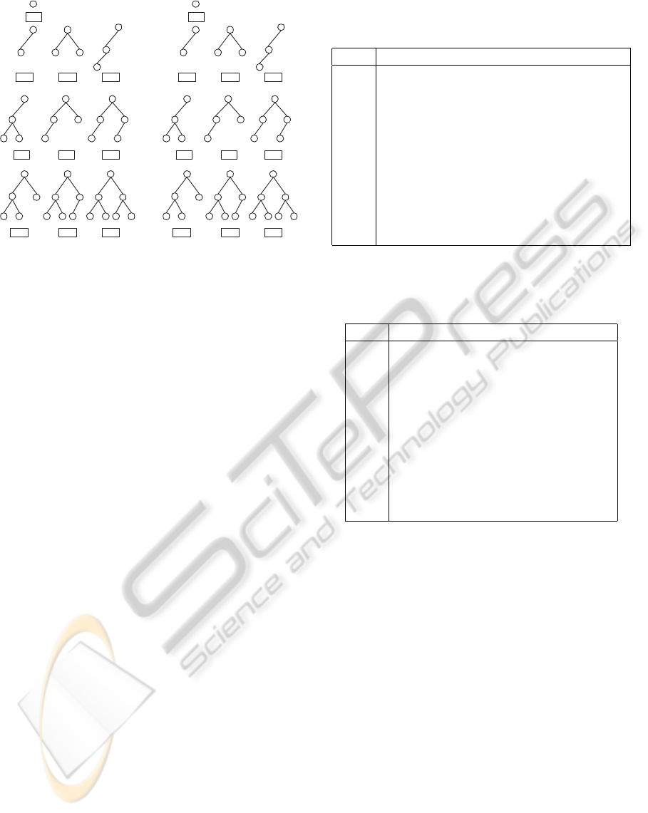
3 - 3
3 - 4 4 - 4 4 - 4
5 - 5 5 - 5 6 - 6
6 - 6 7 - 7 8 - 8
3 - 3
4 - 5 6 - 6 4 - 5
5 - 5 6 - 7 6 - 7
7 - 7 7 - 8 8 - 8
(a) (b)
Figure 6: Calculated lower bound and the exact VC-
dimension of univariate decision trees for datasets with 3
(a) and 4 (b) input features. Only the internal nodes are
shown.
4.2 Complexity Control using
VC-Dimension Bounds
In this section to show that our VC-dimension bounds
are useful, we use them for complexity control in de-
cision trees. Controlling complexity in decision trees
could be done in two ways. We can control the com-
plexities of the decision nodes by selecting the appro-
priate model for a node (Yıldız and Alpaydın, 2001),
or we can control the overall complexity of the de-
cision tree via pruning. Since this paper covers only
discrete univariate trees, we take the second approach
and use the VC-dimension bounds found in the previ-
ous section for pruning.
When we prune a node using SRM (SRMprune),
we first find the VC generalization error using Equa-
tion 2 where V is the VC-dimension and E
t
is the
training error of the subtree. Then, we find the train-
ing error of the node as if it is a leaf node. Since
the VC-dimension of a leaf node is 1, we can find
the generalization error of the tree as if it is pruned.
If the generalization error of the leaf node is smaller
than the generalization error of the subtree, we prune
the subtree, otherwise we keep it. We compare SRM
based pruning with CVprune, where we evaluate the
performance of the subtree with a leaf replacing the
subtree on a separate validation set. For the sake of
generality, we also include the results of trees be-
fore any pruning is applied (NOprune). We use a
total of 11 data sets where 9 of them are (artificial,
krvskp, monks, mushroom, promoters, spect, tictac-
toe, titanic, and vote) from UCI repository (Blake
and Merz, 2000) and 2 are (acceptors and donors)
Table 1: The average and standard deviations of error rates
of decision trees generated using NOprune, CVprune, and
SRMprune.
Set NOprune CVprune SRMprune
Acc 17.1 ± 1.6 15.5 ± 2.3 15.6 ± 1.6
Art 0.0 ± 0.0 0.5 ± 1.4 0.0 ± 0.0
Don 8.0 ± 1.1 7.1 ± 1.1 6.7 ± 1.1
Krv 0.3 ± 0.3 1.2 ± 0.7 0.6 ± 0.4
Mon 4.2 ± 5.9 10.0 ± 7.6 4.2 ± 5.9
Mus 0.0 ± 0.0 0.0 ± 0.1 0.0 ± 0.0
Pro 23.6 ± 12.5 24.7 ± 12.9 20.6 ± 12.3
Spe 25.4 ± 7.9 20.9 ± 3.6 22.1 ± 7.1
Tic 14.2 ± 3.8 18.5 ± 4.2 14.2 ± 3.8
Tit 21.0 ± 1.7 21.5 ± 2.1 22.6 ± 2.1
Vot 6.3 ± 3.6 4.4 ± 2.9 3.9 ± 3.4
Table 2: The average and standard deviations of tree
complexities of decision trees generated using NOprune,
CVprune, and SRMprune.
Set NOprune CVprune SRMprune
Acc 1015 ± 29 55 ± 42 838 ± 31
Art 16 ± 0 15 ± 2 16 ± 0
Don 1489 ± 32 145 ± 35 910 ± 74
Krv 138 ± 6 80 ± 13 122 ± 9
Mon 121 ± 50 57 ± 17 121 ± 50
Mus 43 ± 0 41 ± 4 43 ± 0
Pro 48 ± 5 13 ± 6 39 ± 3
Spe 165 ± 9 5 ± 10 60 ± 16
Tic 437 ± 31 123 ± 25 436 ± 31
Tit 32 ± 1 16 ± 4 5 ± 2
Vot 89 ± 8 9 ± 8 23 ± 8
bioinformatics datasets. We use 10×10 fold cross-
validation to generate training and test sets. For
CVprune, 20 percent of the training data is put aside
as the pruning set. for SRMprune we did a grid-search
on a
1
and a
2
using cross-validation and used a
1
= 0.1
and a
2
= 2.0.
Tables 1 and 2 show the average and standard de-
viations of error rates and tree complexities of deci-
sion trees generated using NOprune, CVprune, and
SRMprune respectively. On four datasets (artificial,
monks, mushroom, and tictactoe) there is no need to
prune, i.e., pruning decreases performance and in this
cases, CVprune prunes trees aggressively by sacrific-
ing from accuracy,whereas SRMprune does not prune
and gets the best performance with NOprune.
On five datasets (acceptors, donors, spect, pro-
moters, and vote) pruning helps, i.e., pruning both re-
duces both the error rate and the tree complexity as
needed. For those datasets, on two datasets CVprune
is better than SRMprune, whereas on three datasets
SRMprune is better than CVprune.
On two datasets (titanic and krvskp), both
ON THE VC-DIMENSION OF UNIVARIATE DECISION TREES
209

CVprune and SRMprune prune more than needed and
therefore can not decrease error rate. In general,
CVprune prunes more aggresively than SRMprune
which can cause a decrease in performance.
5 CONCLUSIONS
This paper tries to fill the gap in the statistical learning
theory, where there is no explicit formula for the VC-
dimension of a decision tree. In this work, we first
focused on the easiest case of univariate trees with bi-
nary features. Starting from basic decision tree with a
single decision node, we give and prove lower bounds
of the VC-dimension of different decision tree struc-
tures. We also prove that the VC-dimension of a uni-
variate decision tree with binary features depends on
the number of features and the VC-dimension of the
left and right subtrees of it (tree structure).
We use the exhaustive search algorithm given
in (Aslan et al., 2009) to calculate the exact VC-
dimension of simple trees and compare our bounds
with the exact VC-dimension values, where the re-
sults show that our bounds are tight. These VC-
dimension bounds are then used in pruning us-
ing SRM and when compared with cross-validation
pruning, we see that SRM pruning using our VC-
dimension values work well and find trees that are
as accurate as CV pruning without the overhead of
cross-validation or needing to leave out some data for
training set.
REFERENCES
Aslan, O., Yıldız, O. T., and Alpaydın, E. (2009). Calculat-
ing the vc-dimension of decision trees. In Proceedings
of the 24th International Symposium on Computer and
Information Sciences, pages 193–198.
Bishop, C. M. (1995). Neural Networks for Pattern Recog-
nition. Oxford University Press.
Blake, C. and Merz, C. (2000). UCI repository of machine
learning databases.
Cherkassky, V. and Mulier, F. (1998). Learning From Data.
John Wiley and Sons.
Mansour, Y. (1997). Pessimistic decision tree pruning based
on tree size. In Proceedings of the 14th international
conference on Machine learning.
Quinlan, J. R. (1986). Induction of decision trees. Machine
Learning, 1:81–106.
Quinlan, J. R. (1993). C4.5: Programs for Machine Learn-
ing. Morgan Kaufmann, San Meteo, CA.
Simon, H. U. (1991). The vapnik-chervonenkis dimension
of decision trees with bounded rank. Information Pro-
cessing Letters, 39(3):137–141.
Vapnik, V. (1995). The Nature of Statistical Learning The-
ory. Springer Verlag, New York.
Yıldız, O. T. and Alpaydın, E. (2001). Omnivariate deci-
sion trees. IEEE Transactions on Neural Networks,
12(6):1539–1546.
ICPRAM 2012 - International Conference on Pattern Recognition Applications and Methods
210
