COST SENSITIVE AND PREPROCESSING FOR CLASSIFICATION

WITH IMBALANCED DATA-SETS: SIMILAR BEHAVIOUR

AND POTENTIAL HYBRIDIZATIONS

Victoria L´opez

, Alberto Fern´andez

, Mar´ıa Jos´e del Jesus

and Francisco Herrera

Dept. of Computer Science and Artiﬁcial Intelligence, CITIC-UGR (Research Center on Information

and Communications Technology), University of Granada, 18071 Granada, Spain

Dept. of Computer Science, University of Ja´en, Ja´en, Spain

Keywords:

Classiﬁcation, Imbalanced data-sets, Preprocessing, Sampling, Cost-sensitive learning, Hybridizations.

Abstract:

The scenario of classiﬁcation with imbalanced data-sets has supposed a serious challenge for researchers along

the last years. The main handicap is related to the large number of real applications in which one of the classes

of the problem has a few number of examples in comparison with the other class, making it harder to be cor-

rectly learnt and, what is most important, this minority class is usually the one with the highest interest.

In order to address this problem, two main methodologies have been proposed for stressing the signiﬁcance of

the minority class and for achieving a good discrimination for both classes, namely preprocessing of instances

and cost-sensitive learning. The former rebalances the instances of both classes by replicating or creating new

instances of the minority class (oversampling) or by removing some instances of the majority class (undersam-

pling); whereas the latter assumes higher misclassiﬁcation costs with samples in the minority class and seek

to minimize the high cost errors. Both solutions have shown to be valid for dealing with the class imbalance

problem but, to the best of our knowledge, no comparison between both approaches have ever been performed.

In this work, we carry out a full exhaustive analysis on this two methodologies, also including a hybrid pro-

cedure that tries to combine the best of these models. We will show, by means of a statistical comparative

analysis developed with a large collection of more than 60 imbalanced data-sets, that we cannot highlight an

unique approach among the rest, and we will discuss as a potential research line the use of hybridizations for

achieving better solutions to the imbalanced data-set problem.

1 INTRODUCTION

In many supervised learning applications, there is a

signiﬁcant difference between the class prior rates,

that is the probability a particular example belongs

to a particular class. This situation is known as the

class imbalance problem (Chawla et al., 2004; Sun

et al., 2009; He and Garcia, 2009) and it is domi-

nant in a high number of real problems including, but

not limited to, telecommunications, WWW, ﬁnances,

ecology, biology, medicine and so on; for which it is

considered as one of the top problems in data min-

ing (Yang and Wu, 2006). Furthermore, it is worth to

point out that the positive or minority class is usually

the one that has the highest interest from the learning

point of view and it also implies a great cost when it

is not well classiﬁed (Elkan, 2001).

The hitch with imbalanced data-sets is that stan-

dard classiﬁcation learning algorithms are often bi-

ased towards the majority classes and therefore there

is a higher misclassiﬁcation rate in the minority class

instances. Therefore, throughout the last years, many

solutions have been proposed to deal with this prob-

lem, which can be categorized into two major groups:

1. Data Sampling: in which the training instances

are modiﬁed in such a way as to produce a more

balanced class distribution that allow classiﬁers to

perform in a similar manner to standard classiﬁ-

cation (Batista et al., 2004; Chawla et al., 2002).

2. Algorithmic Modiﬁcation: this procedure is ori-

ented towards the adaptation of base learning

methods to be more attuned to class imbalance is-

sues (Zadrozny and Elkan, 2001). We must also

stress in this case the use of cost-sensitive learning

solutions, which basically assume higher misclas-

siﬁcation costs with samples in the rare class and

seek to minimize the high cost errors (Domingos,

López V., Fernández A., José del Jesus M. and Herrera F. (2012).

COST SENSITIVE AND PREPROCESSING FOR CLASSIFICATION WITH IMBALANCED DATA-SETS: SIMILAR BEHAVIOUR AND POTENTIAL

HYBRIDIZATIONS.

In Proceedings of the 1st International Conference on Pattern Recognition Applications and Methods, pages 98-107

DOI: 10.5220/0003751600980107

 SciTePress

1999; Zadrozny et al., 2003).

Works in imbalanced classiﬁcation usually focus

on the development of new algorithms along one of

the categories previously mentioned. However, there

is not a study that exhaustively compares solutions

from one category to another making difﬁcult the se-

lection of one kind of algorithm when classifying.

The aim of this contribution is to develop a thorough

experimental study to analyze the possible differences

between preprocessing techniques and cost-sensitive

learning for addressing classiﬁcation with imbalanced

data. In addition, we also present in the comparison a

hybrid procedure that combines those two approaches

to check whether there is a synergy between them.

As baseline classiﬁer, we will use the C4.5 deci-

sion tree generating algorithm (Quinlan, 1993); ﬁrstly

because it has been widely used to deal with imbal-

anced data-sets (Su and Hsiao, 2007; Drown et al.,

2009; Garc´ıa et al., 2009), and secondly since it has

been included as one of the top-ten data-mining algo-

rithms (Wu and Kumar, 2009).

In order to analyze the oversampling and under-

sampling methodologies, we will focus on two of the

most robust approaches such as the “Synthetic Mi-

nority Over-sampling TEchnique”(SMOTE) (Chawla

et al., 2002) and its variant with the Wilson’s Edited

Nearest Neighbour (ENN) rule (Wilson, 1972), as

suggested by their performance among many differ-

ent situations (Batista et al., 2004; Fern´andez et al.,

2008). Regarding cost-sensitive methods, we have

selected the C4.5-CS algorithm (Ting, 2002), which

modiﬁes the computation of the split criteria for C4.5

(normalized information gain) to take into account the

a priori probabilities according to the number of sam-

ples for each class.

In this work, we focus on imbalanced binary clas-

siﬁcation problems, having selected a benchmark of

66 problems from KEEL data-set repository

(Alcal´a-

Fdez et al., 2011). We perform our experimental study

focusing on the precision of the models using the

Area Under the ROC curve (AUC) (Huang and Ling,

2005). This study is carried out using nonparamet-

ric tests to check whether there exist signiﬁcant dif-

ferences among the obtained results (Demˇsar, 2006;

Garc´ıa and Herrera, 2008).

This contribution is organized as follows: ﬁrst,

Section 2 presents the problem of imbalanced data-

sets and the metric we have employed in this context

whereas Section 3 describes the main methodologies

to address the problem: the preprocessing methods

used, cost-sensitive classiﬁcation and a wrapper ap-

proach to combine both. In Section 4 an analysis of

http://www.keel.es/data-sets.php

preprocessing techniques versus cost-sensitive learn-

ing approaches can be found. Finally, the conclusions

of this work are commented in Section 5.

2 IMBALANCED DATA-SETS IN

CLASSIFICATION

In this section, we ﬁrst introduce the problem of im-

balanced data-sets and then we present the evaluation

metrics for this type of classiﬁcation problem which

differs from usual measures in classiﬁcation.

2.1 The Problem of Imbalanced

Data-sets

In the classiﬁcation problem ﬁeld, the scenario of

imbalanced data-sets appears frequently. The main

property of this type of classiﬁcation problem is that

the examples of one class outnumber the examples

of the other one (Japkowicz and Stephen, 2002; Guo

et al., 2008; Sun et al., 2009; He and Garcia, 2009).

The minority class usually represents the most impor-

tant concept to be learnt, since it might be associated

with exceptional and signiﬁcant cases (Weiss, 2004),

or because the data acquisition of these examples is

costly (Weiss and Tian, 2008).

Since most of the standard learning algorithms

consider a balanced training set, this situation may

cause the obtention of suboptimal classiﬁcation mod-

els, i.e. a good coverage of the majority exam-

ples whereas the minority ones are misclassiﬁed fre-

quently; therefore, those algorithms which obtains a

good behaviour in the framework of standard clas-

siﬁcation do not necessarily achieves the best per-

formance for imbalanced data-sets (Fernandez et al.,

2010). There are several reasons behind this be-

haviour which are enumerated below:

1. The use of global performance measures for guid-

ing the search process, such as standard accuracy

rate, may beneﬁt the covering of the majority ex-

amples.

2. Classiﬁcation rules that predict the positive class

are often highly specialized and thus their cover-

age is very low, hence they are discarded in favour

of more general rules, i.e. those that predict the

negative class.

3. It is always difﬁcult to distinguish between noise

examples and minority class examples and they

can be completely ignored by the classiﬁer.

In recent years, the imbalanced learning problem

has received a high attention in the machine learn-

COST SENSITIVE AND PREPROCESSING FOR CLASSIFICATION WITH IMBALANCED DATA-SETS: SIMILAR

BEHAVIOUR AND POTENTIAL HYBRIDIZATIONS

ing community. Speciﬁcally, regarding real world do-

mains the importance of the imbalance learning prob-

lem is growing, since it is a recurring problem in

many applications. As a few examples, we may ﬁnd

very high resolution airbourne imagery (Chen et al.,

2011), face recognition (Kwak, 2008) and especially

medical diagnosis (Lo et al., 2008; Mazurowski et al.,

2008). It is important to remember that the minority

class usually represents the concept of interest and it

is the most difﬁcult to obtain from real data, for ex-

ample patients with illnesses in a medical diagnosis

problem; whereas the other class represents the coun-

terpart of that concept (healthy patients).

2.2 Evaluation in Imbalanced Domains

The evaluation criteria is a key factor in both assess-

ing the classiﬁcation performance and guiding the

classiﬁer modelling. In a two-class problem, the con-

fusion matrix (shown in Table 1) records the results

of correctly and incorrectly recognized examples of

each class.

Table 1: Confusion matrix for a two-class problem.

Positive prediction Negative prediction

Positive class True Positive (TP) False Negative (FN)

Negative class False Positive (FP) True Negative (TN)

Traditionally, accuracy rate (Eq. (1)) has been the

most commonly used empirical measure. However, in

the frameworkof imbalanced data-sets, accuracyis no

longer a proper measure, since it does not distinguish

between the number of correctly classiﬁed examples

of different classes. Hence, it may lead to erroneous

conclusions, i.e., a classiﬁer achieving an accuracy of

90% in a data-set with an IR value of 9, is not accurate

if it classiﬁes all examples as negatives.

Acc =

TP+ TN

TP+ FN + FP + TN

(1)

According to the previous issue, in this work we

use the Area Under the Curve (AUC) metric (Huang

and Ling, 2005), which can be deﬁned as

AUC =

1+ TP

rate

− FP

rate

(2)

where TP

rate

is the percentage of positive cases cor-

rectly classiﬁed as belonging to the positive class and

rate

is the percentage of negative cases misclassi-

ﬁed as belonging to the positive class.

3 ADDRESSING

CLASSIFICATION WITH

IMBALANCED DATA:

PREPROCESSING AND

COST-SENSITIVE LEARNING

A large number of approaches have been proposed

to deal with the class imbalance problem. These ap-

proaches can be categorized into two groups: the in-

ternal approaches that create new algorithms or mod-

ify existing ones to take the class-imbalance problem

into consideration (Barandela et al., 2003; Sun et al.,

2007; Ducange et al., 2010) and external approaches

that preprocess the data in order to diminish the ef-

fect of their class imbalance (Batista et al., 2004; Es-

tabrooks et al., 2004).

Regarding this, in this section we ﬁrst intro-

duce the main features of preprocessing techniques,

focusing on SMOTE (Chawla et al., 2002) and

SMOTE+ENN (Batista et al., 2004), which will be

used along the experimental study. Next, we describe

cost-sensitive learning and the C4.5-CS methodology

(Ting, 2002). Finally, we present a framework to au-

tomatically detect a threshold for preprocessing using

an underlying algorithm, in this case, a cost-sensitive

approach.

3.1 Preprocessing Imbalanced

Data-sets: Resampling Techniques

In the specialized literature, we can ﬁnd some pa-

pers about resampling techniques studying the effect

of changing the class distribution to deal with imbal-

anced data-sets.

Those works have proved empirically that, apply-

ing a preprocessing step in order to balance the class

distribution, is usually an useful solution (Batista

et al., 2004; Fern´andez et al., 2008; Fern´andez et al.,

2010). Furthermore, the main advantage of these

techniques is that they are independent of the under-

lying classiﬁer.

Resampling techniques can be categorized into

three groups or families:

1. Undersampling Methods, which create a subset

of the original data-set by eliminating instances

(usually majority class instances).

2. Oversampling Methods, which create a superset

of the original data-set by replicating some in-

stances or creating new instances from existing

ones.

3. Hybrids Methods, which combine both sampling

approaches.

ICPRAM 2012 - International Conference on Pattern Recognition Applications and Methods

100

Among these categories, there are several propos-

als where the simplest preprocessing are non heuristic

methods such as random undersampling and random

oversampling. In the ﬁrst case, the major drawback is

that it can discard potentially useful data, that could

be important for the induction process. For random

oversampling, several authors agree that this method

can increase the likelihood of occurring overﬁtting,

since it makes exact copies of existing instances.

According to the previous facts, more sophisti-

cated methods have been proposed. Among them,

SMOTE (Chawla et al., 2002) has become one of the

most renowned approaches in this area. In brief, its

main idea is to create new minority class examples by

interpolating several minority class instances that lie

together for oversampling the training set.

With this technique, the positive class is over-

sampled by taking each minority class sample and in-

troducing synthetic examples along the line segments

joining any/all of the k minority class nearest neigh-

bours. Depending upon the amount of over-sampling

required, neighbours from the k nearest neighbours

are randomly chosen. This process is illustrated in

Figure 1, where x

is the selected point, x

to x

are

some selected nearest neighbours and r

to r

the syn-

thetic data points created by the randomized interpo-

lation.

Figure 1: An illustration of how to create the synthetic data

points in the SMOTE algorithm.

However, in oversampling techniques, and espe-

cially for the SMOTE algorithm, the problem of over

generalization is largely attributed to the way in which

it creates synthetic samples. Speciﬁcally, SMOTE

generates the same number of synthetic data samples

for each original minority example and does so with-

out consideration to neighboring examples, which in-

creases the occurrenceof overlapping between classes

(Wang and Japkowicz, 2004). For this reason we also

consider a hybrid approach in this work, “SMOTE +

ENN”, where the Wilson’s ENN Rule (Wilson, 1972)

is used after the SMOTE application to remove from

the training set any example misclassiﬁed by its three

nearest neighbours.

3.2 Cost-sensitive Learning

Cost-sensitive learning takes into account the vari-

able cost of a misclassiﬁcation of the different classes

(Domingos, 1999; Zadrozny et al., 2003). In this case,

a cost matrix codiﬁes the penalties C(i, j) of classify-

ing examples of one class as a different one; if we use

the notation 1 for minority and 0 for majority class,

C(i, i) = TN or TP. These misclassiﬁcation cost val-

ues can be given by domain experts, or learned via

other approaches (Sun et al., 2009; Sun et al., 2007).

Speciﬁcally, when dealing with imbalanced problems

it is usually of most interest to recognize the posi-

tive instances rather than the negative ones and there-

fore, the cost when misclassifying a positive instance

is higher than the cost of misclassifying a negative

one.

Given the cost matrix, an example should be clas-

siﬁed into the class that has the minimum expected

cost. This is the minimum expected cost principle.

The expected cost R(i|x) of classifying an instance x

into class i (by a classiﬁer) can be expressed as:

R(i|x) =

∑

P( j|x) ·C(i, j) (3)

where P( j|x) is the probability estimation of classify-

ing an instance into class j. That is, the classiﬁer will

classify an instance x into positive class if and only if:

P(0|x)·(C(1, 0)−C(0, 0)) ≤ P(1|x)(C(0, 1)−C(1, 1))

Therefore, any given cost-matrix can be converted

to one withC(0, 0) = C(1, 1) = 0. Under this assump-

tion, the classiﬁer will classify an instance x into pos-

itive class if and only if:

P(0|x) ·C(1, 0) ≤ P(1|x) ·C(0, 1)

As P(0|x) = 1 − P(1|x), we can obtain a thresh-

old p

∗

for the classiﬁer to classify an instance x into

positive if P(1|x) ≥ p

∗

, where

∗

C(1, 0)

C(1, 0) −C(0, 1)

FP+ FN

(4)

Another possibility is to “rebalance” the original

training examples the ratio of:

p(1)FN : p(0)FP (5)

where p(1) and p(0) are the prior probability of the

positive and negative examples in the original training

set.

In summary, two main general approaches have

been proposed to deal with cost-sensitive problems:

COST SENSITIVE AND PREPROCESSING FOR CLASSIFICATION WITH IMBALANCED DATA-SETS: SIMILAR

BEHAVIOUR AND POTENTIAL HYBRIDIZATIONS

101

1. Direct Methods: The main idea of building a di-

rect cost-sensitive learning algorithm is to directly

introduce and utilize misclassiﬁcation costs into

the learning algorithms.

For example, in the context of decision tree in-

duction, the tree-building strategies are adapted

to minimize the misclassiﬁcation costs. The cost

information is used to: (1) choose the best at-

tribute to split the data (Ling et al., 2004; Riddle

et al., 1994); and (2) determine whether a sub-

tree should be pruned (Bradford et al., 1998). On

the other hand, other approaches based on genetic

algorithms can incorporate misclassiﬁcation costs

in the ﬁtness function (Turney, 1995).

2. Meta-learning: This methodology implies the in-

tegration of a “preprocessing” mechanism for the

training data or a “postprocessing” of the out-

put, in such a way that the original learning al-

gorithm is not modiﬁed. Cost-sensitive meta-

learning can be further classiﬁed into two main

categories: thresholding and sampling, which are

based on expressions (4) and (5) respectively:

• Thresholding is based on the Bayes decision

theory that assign instances to the class with

minimum expected cost, as introduced above.

For example, a typical decision tree for a binary

classiﬁcation problem assigns the class label of

a leaf node depending on the majority class of

the training samples that reach the node. A

cost-sensitive algorithm assigns the class label

to the node that minimizes the classiﬁcation

cost (Domingos, 1999; Zadrozny and Elkan,

2001).

• Sampling is based on modifying the train-

ing data-set. The most popular technique

lies in resampling the original class distribu-

tion of the training data-set according to the

cost decision matrix by means of undersam-

pling/oversampling (Zadrozny et al., 2003) or

assigning instance weights (Ting, 2002). These

modiﬁcations have shown to be effective and

can also be applied to any cost insensitivelearn-

ing algorithm (Zhou and Liu, 2006).

In this work, we will make use of the cost-

sensitive C4.5 decision tree (C4.5-CS) proposed in

(Ting, 2002). This method changes the class distri-

bution such that the tree induced is in favor of the

class with high weight/cost and is less likely to com-

mit errors with high cost. Speciﬁcally, the computa-

tion of the split criteria for C4.5 (normalized informa-

tion gain) is modiﬁed to take into account the a priori

probabilities according to the number of samples for

each class.

The standard greedy divide-and-conquer proce-

dure for inducing minimum error trees can then be

used without modiﬁcation, except that W

(t) (6) is

used instead of N

(t) (number of instances of class

j) in the computation of the test selection criterion in

the tree growing process and the error estimation in

the pruning process.

W( j) = C( j)

∑

C(i)N

(6)

C4.5-CS also introduces another optional modiﬁ-

cation that alters the usual classiﬁcation process after

creating the decision tree. Instead of classifying us-

ing the minimum error criteria, it is advisable to clas-

sify using the expected misclassiﬁcation cost in the

last part of the classiﬁcation procedure. The expected

misclassiﬁcation cost for predicting class i with re-

spect to the instance x is given by

(x) ∝

∑

(t(x))cost(i, j) (7)

where t(x) is the leaf of the tree that instance x

falls into and W

(t) is the total weight of class j train-

ing instances in node t.

3.3 Hybridization. Automatically

Countering Imbalance

The different solutions used to deal with the imbal-

anced problem have been presented in the previous

subsections. So the question now is “Can we use both

techniques together and achieve better results?”.

In this section we describe a procedure to inte-

grate the cost-sensitivelearning and preprocessing ap-

proaches into one, quite similar to the one proposed

in (Chawla et al., 2008), which consists in a wrap-

per paradigm that discovers the amount of resampling

needed for a data-set based on optimizing evaluation

functions which can include the cost associated to

the classiﬁcation. This wrapper infrastructure applies

cross-validation to ﬁrst discover the best amounts of

undersampling and oversampling, applies the prepro-

cessing algorithms with the amounts estimated and ﬁ-

nally runs the algorithm used over the preprocessed

data-set. Figure 2 shows the algorithm procedure.

The undersampling estimation starts with no un-

dersampling for all majority classes and obtains base-

line results on the training data. Then it traverses

through the search space of undersampling percent-

ages in decrements of Sample Decrement (in this case

10%), in a greedy iterative fashion, to increase perfor-

mance over the minority classes without sacriﬁcing

performance on the majority class.

ICPRAM 2012 - International Conference on Pattern Recognition Applications and Methods

102

Figure 2: Illustration on the Wrapper Undersample SMOTE Algorithm. Dashed lines means resampling actions, black boxes

represent the parameters estimation and the ﬁnal result is in grey.

The oversampling algorithm evaluates different

amounts of SMOTE at steps of 100% (the num-

ber of examples from the minority class). This is

a greedy search, and at each step the new perfor-

mance estimates become the new baseline. That is,

the initial baseline is the performance obtained via the

Wrapper Undersample. If SMOTE=100% improves

the performance over that baseline by some mar-

gin Increment Min, then the performance achieved

at SMOTE=100% becomes the new baseline. The

amount of SMOTE is then incremented by Sample In-

crement, and another evaluationis performed to check

if the performance increase at new SMOTE amount

is at least greater than Increment Min. This process

repeats, greedily, until no performance gains are ob-

served.

However,there is an importantcaveat to the search

to avoid being trapped in a local maximum. If the av-

erage does not improve by 5% we have to verify that

we have not settled on a local maximum. In order

to do so, we look ahead two more steps at increas-

ing amounts of SMOTE. If the look-ahead does not

result in an improvement in performance, then the

amount of SMOTE is reset to the value discovered

prior to the look-ahead. This is done to allow SMOTE

to introduce additional examples with the aim of im-

proving performance. However, if the addition of ex-

amples does not help, then we go back to using the

lesser amountof SMOTE discovered prior to the look-

ahead.

We can use different measures to evaluate the per-

formance of the classiﬁer to estimate the sampling pa-

rameters. In our case, different from (Chawla et al.,

2008), we use cost-sensitive learning algorithms as

base classiﬁers, and therefore a logical evaluation cri-

teria is the cost itself. Cost is calculated as shown in

Equation 8 when we assume C(+|+) = C(−|−) = 0

(as it is usual in imbalanced classiﬁcation).

cost = FNrate ·C(−|+) + FPrate×C(+|−) (8)

4 EXPERIMENTAL STUDY

In this section, we will perform an analysis to de-

termine the performance of the different alternatives

used for imbalanced classiﬁcation. Our aim is to ana-

lyze three different issues:

1. The improvementobtained by preprocessing data-

sets and cost-sensitive learning over the original

algorithm.

2. The possible differences between the rebalancing

techniques versus cost-sensitive learning and in

which cases.

3. Whether a hybrid methodology that combines a

preprocessing approach and a cost-sensitive learn-

ing algorithm supposes a positive synergy and en-

ables the achievement of more accurate results.

First, we present our experimental framework

with the data-set employed in our analysis and the

statistical tests that will allow us to support the ex-

tracted ﬁndings. Then, we will show the results from

our study and we will discuss the main issues that will

arise from the aforementioned analysis.

4.1 Experimental Framework

In order to analyze the preprocessing approach

against the cost-sensitive learning strategy, we have

selected 66 data-sets from the KEEL data-set reposi-

tory

(Alcal´a-Fdez et al., 2011). These data-sets are

summarized in Table 2, where we denote the num-

ber of examples (#Ex.), number of attributes (#Atts.),

class name of each class (positive and negative), class

distribution and IR.

To develop the different experiments we consider

a 5-folder cross-validation model, i.e., ﬁve random

partitions of data with a 20% and the combination of

http://www.keel.es/data-sets.php

COST SENSITIVE AND PREPROCESSING FOR CLASSIFICATION WITH IMBALANCED DATA-SETS: SIMILAR

BEHAVIOUR AND POTENTIAL HYBRIDIZATIONS

103

Table 2: Summary of imbalanced data-sets.

Data-sets #Ex. #Atts. Class (-,+) %Class(-; +) IR

Glass1 214 9 (build-win-non ﬂoat-proc; remainder) (35.51, 64.49) 1.82

Ecoli0vs1 220 7 (im; cp) (35.00, 65.00) 1.86

Wisconsin 683 9 (malignant; benign) (35.00, 65.00) 1.86

Pima 768 8 (tested-positive; tested-negative) (34.84, 66.16) 1.90

Iris0 150 4 (Iris-Setosa; remainder) (33.33, 66.67) 2.00

Glass0 214 9 (build-win-ﬂoat-proc; remainder) (32.71, 67.29) 2.06

Yeast1 1484 8 (nuc; remainder) (28.91, 71.09) 2.46

Vehicle1 846 18 (Saab; remainder) (28.37, 71.63) 2.52

Vehicle2 846 18 (Bus; remainder) (28.37, 71.63) 2.52

Vehicle3 846 18 (Opel; remainder) (28.37, 71.63) 2.52

Haberman 306 3 (Die; Survive) (27.42, 73.58) 2.68

Glass0123vs456 214 9 (non-window glass; remainder) (23.83, 76.17) 3.19

Vehicle0 846 18 (Van; remainder) (23.64, 76.36) 3.23

Ecoli1 336 7 (im; remainder) (22.92, 77.08) 3.36

New-thyroid2 215 5 (hypo; remainder) (16.89, 83.11) 4.92

New-thyroid1 215 5 (hyper; remainder) (16.28, 83.72) 5.14

Ecoli2 336 7 (pp; remainder) (15.48, 84.52) 5.46

Segment0 2308 19 (brickface; remainder) (14.26, 85.74) 6.01

Glass6 214 9 (headlamps; remainder) (13.55, 86.45) 6.38

Yeast3 1484 8 (me3; remainder) (10.98, 89.02) 8.11

Ecoli3 336 7 (imU; remainder) (10.88, 89.12) 8.19

Page-blocks0 5472 10 (remainder; text) (10.23, 89.77) 8.77

Ecoli034vs5 200 7 (p,imL,imU; om) (10.00, 90.00) 9.00

Yeast2vs4 514 8 (cyt; me2) (9.92, 90.08) 9.08

Ecoli067vs35 222 7 (cp,omL,pp; imL,om) (9.91, 90.09) 9.09

Ecoli0234vs5 202 7 (cp,imS,imL,imU; om) (9.90, 90.10) 9.10

Glass015vs2 172 9 (build-win-non

ﬂoat-proc,tableware, (9.88, 90.12) 9.12

build-win-ﬂoat-proc; ve-win-ﬂoat-proc)

Yeast0359vs78 506 8 (mit,me1,me3,erl; vac,pox) (9.88, 90.12) 9.12

Yeast02579vs368 1004 8 (mit,cyt,me3,vac,erl; me1,exc,pox) (9.86, 90.14) 9.14

Yeast0256vs3789 1004 8 (mit,cyt,me3,exc; me1,vac,pox,erl) (9.86, 90.14) 9.14

Ecoli046vs5 203 6 (cp,imU,omL; om) (9.85, 90.15) 9.15

Ecoli01vs235 244 7 (cp,im; imS,imL,om) (9.83, 90.17) 9.17

Ecoli0267vs35 224 7 (cp,imS,omL,pp; imL,om) (9.82, 90.18) 9.18

Glass04vs5 92 9 (build-win-ﬂoat-proc,containers; tableware) (9.78, 90.22) 9.22

Ecoli0346vs5 205 7 (cp,imL,imU,omL; om) (9.76, 90.24) 9.25

Ecoli0347vs56 257 7 (cp,imL,imU,pp; om,omL) (9.73, 90.27) 9.28

Yeast05679vs4 528 8 (me2; mit,me3,exc,vac,erl) (9.66, 90.34) 9.35

Ecoli067vs5 220 6 (cp,omL,pp; om) (9.09, 90.91) 10.00

Vowel0 988 13 (hid; remainder) (9.01, 90.99) 10.10

Glass016vs2 192 9 (ve-win-ﬂoat-proc; build-win-ﬂoat-proc, (8.89, 91.11) 10.29

build-win-non

ﬂoat-proc,headlamps)

Glass2 214 9 (Ve-win-ﬂoat-proc; remainder) (8.78, 91.22) 10.39

Ecoli0147vs2356 336 7 (cp,im,imU,pp; imS,imL,om,omL) (8.63, 91.37) 10.59

Led7digit02456789vs1 443 7 (0,2,4,5,6,7,8,9; 1) (8.35, 91.65) 10.97

Glass06vs5 108 9 (build-win-ﬂoat-proc,headlamps; tableware) (8.33, 91.67) 11.00

Ecoli01vs5 240 6 (cp,im; om) (8.33, 91.67) 11.00

Glass0146vs2 205 9 (build-win-ﬂoat-proc,containers,headlamps, (8.29, 91.71) 11.06

build-win-non

ﬂoat-proc;ve-win-ﬂoat-proc)

Ecoli0147vs56 332 6 (cp,im,imU,pp; om,omL) (7.53, 92.47) 12.28

Cleveland0vs4 177 13 (0; 4) (7.34, 92.66) 12.62

Ecoli0146vs5 280 6 (cp,im,imU,omL; om) (7.14, 92.86) 13.00

Ecoli4 336 7 (om; remainder) (6.74, 93.26) 13.84

Yeast1vs7 459 8 (nuc; vac) (6.72, 93.28) 13.87

Shuttle0vs4 1829 9 (Rad Flow; Bypass) (6.72, 93.28) 13.87

Glass4 214 9 (containers; remainder) (6.07, 93.93) 15.47

Page-blocks13vs2 472 10 (graphic; horiz.line,picture) (5.93, 94.07) 15.85

Abalone9vs18 731 8 (18; 9) (5.65, 94.25) 16.68

Glass016vs5 184 9 (tableware; build-win-ﬂoat-proc, (4.89, 95.11) 19.44

build-win-non

ﬂoat-proc,headlamps)

Shuttle2vs4 129 9 (Fpv Open; Bypass) (4.65, 95.35) 20.5

Yeast1458vs7 693 8 (vac; nuc,me2,me3,pox) (4.33, 95.67) 22.10

Glass5 214 9 (tableware; remainder) (4.20, 95.80) 22.81

Yeast2vs8 482 8 (pox; cyt) (4.15, 95.85) 23.10

Yeast4 1484 8 (me2; remainder) (3.43, 96.57) 28.41

Yeast1289vs7 947 8 (vac; nuc,cyt,pox,erl) (3.17, 96.83) 30.56

Yeast5 1484 8 (me1; remainder) (2.96, 97.04) 32.78

Ecoli0137vs26 281 7 (pp,imL; cp,im,imU,imS) (2.49, 97.51) 39.15

Yeast6 1484 8 (exc; remainder) (2.49, 97.51) 39.15

Abalone19 4174 8 (19; remainder) (0.77, 99.23) 128.87

4 of them (80%) as training and test. For each data-set

we consider the average results of the ﬁve partitions.

The data-sets used in this study use the partitions pro-

vided by the repository in the imbalanced classiﬁca-

tion data-set section

Furthermore, we have to identify the misclassiﬁ-

cation costs associated to the positive and negative

class for the cost-sensitive learning versions. If we

misclassify a positive sample as a negative one the

associated misclassiﬁcation cost is the IR of the data-

set (C(+, −) = IR) whereas if we misclassify a nega-

tive sample as a positive one the associated cost is 1

http://www.keel.es/imbalanced.php

(C(−, +) = 1). The cost of classifying correctly is 0

(C(+, +) = C(−, −) = 0) because guessing the cor-

rect class should not penalize the built model.

Finally, statistical analysis needs to be carried out

in order to ﬁnd signiﬁcant differences among the re-

sults obtained by the studied methods (Demˇsar, 2006;

Garc´ıa et al., 2009; Garc´ıa et al., 2010). Since

the study is split in parts comparing a group of al-

gorithms, we use non-parametric statistical tests for

multiple comparisons. Speciﬁcally, we use the Iman-

Davenport test (Sheskin, 2006) to detect statistical

differences among a group of results and the Shaf-

fer post-hoc test (Shaffer, 1986) in order to ﬁnd out

which algorithms are distinctive among an n×n com-

parison.

Furthermore, we consider the average ranking of

the algorithms in order to show graphically how good

a method is with respect to its partners. This rank-

ing is obtained by assigning a position to each algo-

rithm depending on its performance for each data-set.

The algorithm which achieves the best accuracy in a

speciﬁc data-set will have the ﬁrst ranking (value 1);

then, the algorithm with the second best accuracy is

assigned rank 2, and so forth. This task is carried out

for all data-sets and ﬁnally an average ranking is com-

puted as the mean value of all rankings.

4.2 Contrasting Preprocessing and

Cost-sensitive Learning in

Imbalanced Data-sets

Table 3 shows the average results in training and test

together with the corresponding standard deviation

for the seven versions of the C4.5 algorithm used in

the study: the base classiﬁer, the base classiﬁer used

overthe preprocessed data-sets, the cost-sensitive ver-

sion of the algorithm and the hybrid versions of it. We

stress in boldface the best results achievedfor the pre-

diction ability of the different techniques.

Table 3: Average table of results using the AUC measure

for the C4.5 variety of algorithms.

Algorithm AUC

AUC

tst

C4.5 0.8774 ± 0.0392 0.7902 ± 0.0804

C4.5 SMOTE 0.9606 ± 0.0142 0.8324 ± 0.0728

C4.5 SENN 0.9471 ± 0.0154 0.8390 ± 0.0772

C4.5CS 0.9679 ± 0.0103 0.8294 ± 0.0758

C4.5 Wr

SMOTE 0.9679 ± 0.0103 0.8296 ± 0.0763

C4.5 Wr

US 0.9635 ± 0.0139 0.8245 ± 0.0760

C4.5 Wr

SENN 0.9083 ± 0.0377 0.8145 ± 0.0712

From this table of results it can be observed that

the highest average value corresponds to preprocess-

ICPRAM 2012 - International Conference on Pattern Recognition Applications and Methods

104

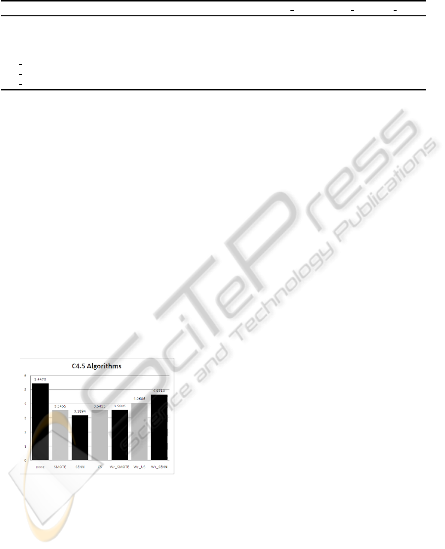
Table 4: Shaffer test for the C4.5 variety of algorithms using the AUC measure.

C4.5 None SMOTE SENN CS Wr SMOTE Wr US Wr SENN

None x -(6.404E-6) -(4.058E-8) -(6.404E-6) -(7.904E-6) -(.00341) =(.37846)

SMOTE +(6.404E-6) x =(1.0) =(1.0) =(1.0) =(1.0) +(.04903)

SENN +(4.058E-8) =(1.0) x =(1.0) =(1.0) =(.22569) +(.00152)

CS +(6.404E-6) =(1.0) =(1.0) x =(1.0) =(1.0) +(.04903)

SMOTE +(7.904E-6) =(1.0) =(1.0) =(1.0) x =(1.0) +(.04903)

US +(.00341) =(1.0) =(.22569) =(1.0) =(1.0) x =(1.0)

SENN =(.37846) -(.04903) -(.00152) -(.04903) -(.04903) =(1.0) x

ing approaches closely followed by the cost-sensitive

learning approach and one version of the wrapper rou-

tine. This suggests the goodness of the preprocessing

and cost-sensitive learning approaches.

In order to compare the results, a multiple com-

parison test is used to ﬁnd the performance relation-

ship between the different versions studied. The re-

sults of the statistical analysis of the C4.5 family are

as follows. For the sake of a visual comparison, Fig-

ure 3 shows the average ranking for these approaches.

Under the AUC measure, the Iman-Davenport test

detects signiﬁcant differences among the algorithms,

since the p-value returned (1.88673E-10) is lower

than our α-value (0.05). The differences found are

analyzed with a Shaffer test, shown in Table 4. In this

table, a “+” symbol implies that the algorithm in the

row is statistically better than the one in the column,

whereas “-” implies the contrary; “=” means that the

two algorithms compared have no signiﬁcant differ-

ences. In brackets, the adjusted p-value associated to

each comparison is shown.

Figure 3: Average rankings using the AUC measure for the

C4.5 variety of algorithms.

Observing the results from Tables 3 and 4, we

conclude that the standard C4.5 approach is out-

performed by most of the methodologies that deal

with imbalanced data. All methodologies, the hy-

brid version that uses only an oversampling step with

SMOTE+ENN, have signiﬁcant differences versus

the base C4.5 classiﬁer. This analysis answers our

ﬁrst question of the study, that is, the classiﬁcation

performance is degraded in an imbalance scenario

having a bias towards the majority class examples and

the use of the aforementioned techniques (preprocess-

ing and cost-sensitive learning) allow us to obtain a

better discrimination of the examples of both classes

resulting in an overall good classiﬁcation for all con-

cepts of the problem (positive and negative classes).

Comparing the results when applying preprocess-

ing we can see that the performance of these meth-

ods is not statistically different for any of its ver-

sions. In addition, the performance of those pre-

processing methods is also not different to the cost-

sensitive learning version of C4.5. This second part

of the study has reﬂected that the two employed so-

lutions are quite similar between them and it was not

possible to highlight one of them as the most adequate

one for classiﬁcation. For that reason, the question on

which approach is preferable for addressing classiﬁ-

cation with imbalanced data-sets is still unresolved.

Finally, regarding the hybridization of cost-

sensitive learning and preprocessing by using a wrap-

per routine, it can be seen that there are signiﬁcant

differences both between the different hybrid versions

and with the other alternatives. The hybrid version

that uses an oversampling step with SMOTE+ENN

is outperformed by all the other versions except the

base version. The rest of the hybrid versions are not

statistically different from the performance of usual

approaches for imbalanced classiﬁcation. Therefore,

we cannot state that the hybridization in decision trees

produces a positive synergy between the two tech-

niques. According to these results, the preliminary

version of the hybrid technique can be further im-

proved both applying a ﬁnest combination of the indi-

vidual approaches or by using more speciﬁc methods

with a better synergy between them.

5 CONCLUSIONS

In this work we have analyzed the behaviour of pre-

processing and cost-sensitive learning in the frame-

work of imbalanced data-sets in order to determine

whether there are any signiﬁcant differences between

COST SENSITIVE AND PREPROCESSING FOR CLASSIFICATION WITH IMBALANCED DATA-SETS: SIMILAR

BEHAVIOUR AND POTENTIAL HYBRIDIZATIONS

105

both approaches and therefore which one of them is

preferred and in which cases. Additionally, we have

proposed a hybrid approach that integrates both ap-

proaches together.

First of all, we have determined that both method-

ologies improve the overall performance for the clas-

siﬁcation with imbalanced data, which was the ex-

pected behaviour. Next, the comparison between pre-

processing techniques against cost-sensitive learning

hints that there are no differences among the differ-

ent preprocessing techniques. The statistical study,

supported by a large collection of more than 60 im-

balanced data-sets, lets us say that both preprocess-

ing and cost-sensitive learning are good and equiva-

lent approaches to address the imbalance problem.

Finally, we have shown that our preliminary ver-

sions of hybridization techniques are truly competi-

tive with the standard methodologies. We must stress

that this is a very interesting trend for research as there

is still room for improvement regarding hybridization

between preprocessing and cost-sensitive learning.

ACKNOWLEDGEMENTS

This work has been supported by the Spanish Min-

istry of Science and Technology under Projects

TIN2011-28488and TIN2008-06681-C06-02and the

Andalusian Research Plans P10-TIC-6858 and TIC-

3928. V. L´opez holds a FPU scholarship from Span-

ish Ministry of Education.

REFERENCES

Alcal´a-Fdez, J., Fern´andez, A., Luengo, J., Derrac, J.,

Garc´ıa, S., S´anchez, L., and Herrera, F. (2011).

KEEL data–mining software tool: Data set repository,

integration of algorithms and experimental analysis

framework. Journal of Multi–Valued Logic and Soft

Computing, 17(2-3):255–287.

Barandela, R., S´anchez, J. S., Garc´ıa, V., and Rangel, E.

(2003). Strategies for learning in class imbalance

problems. Pattern Recognition, 36(3):849–851.

Batista, G. E. A. P. A., Prati, R. C., and Monard, M. C.

(2004). A study of the behaviour of several meth-

ods for balancing machine learning training data.

SIGKDD Explorations, 6(1):20–29.

Bradford, J. P., Kunz, C., Kohavi, R., Brunk, C., and Brod-

ley, C. E. (1998). Pruning decision trees with misclas-

siﬁcation costs. In Proceedings of the 10th European

Conference on Machine Learning (ECML’98), pages

131–136.

Chawla, N. V., Bowyer, K. W., Hall, L. O., and Kegelmeyer,

W. P. (2002). SMOTE: Synthetic minority over–

sampling technique. Journal of Artiﬁcial Intelligent

Research, 16:321–357.

Chawla, N. V., Cieslak, D. A., Hall, L. O., and Joshi,

A. (2008). Automatically countering imbalance and

its empirical relationship to cost. Data Mining and

Knowledge Discovery, 17(2):225–252.

Chawla, N. V., Japkowicz, N., and Kotcz, A. (2004). Edi-

torial: special issue on learning from imbalanced data

sets. SIGKDD Explorations, 6(1):1–6.

Chen, X., Fang, T., Huo, H., and Li, D. (2011). Graph–

based feature selection for object–oriented classiﬁca-

tion in VHR airborne imagery. IEEE Transactions on

Geoscience and Remote Sensing, 49(1):353–365.

Demˇsar, J. (2006). Statistical comparisons of classiﬁers

over multiple data sets. Journal of Machine Learning

Research, 7:1–30.

Domingos, P. (1999). Metacost: A general method for mak-

ing classiﬁers cost–sensitive. In Proceedings of the

5th International Conference on Knowledge Discov-

ery and Data Mining (KDD’99), pages 155–164.

Drown, D. J., Khoshgoftaar, T. M., and Seliya, N. (2009).

Evolutionary sampling and software quality model-

ing of high-assurance systems. IEEE Transactions on

Systems, Man, and Cybernetics, Part A, 39(5):1097–

1107.

Ducange, P., Lazzerini, B., and Marcelloni, F. (2010).

Multi–objective genetic fuzzy classiﬁers for imbal-

anced and cost–sensitive datasets. Soft Computing,

14(7):713–728.

Elkan, C. (2001). The foundations of cost–sensitive learn-

ing. In Proceedings of the 17th IEEE International

Joint Conference on Artiﬁcial Intelligence (IJCAI’01),

pages 973–978.

Estabrooks, A., Jo, T., and Japkowicz, N. (2004). A multi-

ple resampling method for learning from imbalanced

data sets. Computational Intelligence, 20(1):18–36.

Fern´andez, A., del Jesus, M. J., and Herrera, F. (2010).

On the 2–tuples based genetic tuning performance for

fuzzy rule based classiﬁcation systems in imbalanced

data–sets. Information Sciences, 180(8):1268–1291.

Fern´andez, A., Garc´ıa, S., del Jesus, M. J., and Herrera,

F. (2008). A study of the behaviour of linguistic

fuzzy rule based classiﬁcation systems in the frame-

work of imbalanced data–sets. Fuzzy Sets and Sys-

tems, 159(18):2378–2398.

Fernandez, A., Garc´ıa, S., Luengo, J., Bernad´o-Mansilla,

E., and Herrera, F. (2010). Genetics-based machine

learning for rule induction: State of the art, taxonomy

and comparative study. IEEE Transactions on Evolu-

tionary Computation, 14(6):913–941.

Garc´ıa, S., Fern´andez, A., and Herrera, F. (2009). Enhanc-

ing the effectiveness and interpretability of decision

tree and rule induction classiﬁers with evolutionary

training set selection over imbalanced problems. Ap-

plied Soft Computing, 9:1304–1314.

Garc´ıa, S., Fern´andez, A., Luengo, J., and Herrera, F.

(2009). A study of statistical techniques and perfor-

mance measures for genetics–based machine learn-

ing: accuracy and interpretability. Soft Computing,

13(10):959–977.

ICPRAM 2012 - International Conference on Pattern Recognition Applications and Methods

106

Garc´ıa, S., Fern´andez, A., Luengo, J., and Herrera, F.

(2010). Advanced nonparametric tests for multi-

ple comparisons in the design of experiments in

computational intelligence and data mining: Exper-

imental analysis of power. Information Sciences,

180(10):2044–2064.

Garc´ıa, S. and Herrera, F. (2008). An extension on “sta-

tistical comparisons of classiﬁers over multiple data

sets” for all pairwise comparisons. Journal of Ma-

chine Learning Research, 9:2607–2624.

Guo, X., Dong, Y. Y. C., Yang, G., and Zhou, G. (2008).

On the class imbalance problem. In Proceedings of the

4th International Conference on Natural Computation

(ICNC’08), volume 4, pages 192–201.

He, H. and Garcia, E. A. (2009). Learning from imbalanced

data. IEEE Transactions on Knowledge and Data En-

gineering, 21(9):1263–1284.

Huang, J. and Ling, C. X. (2005). Using AUC and accuracy

in evaluating learning algorithms. IEEE Transactions

on Knowledge and Data Engineering, 17(3):299–310.

Japkowicz, N. and Stephen, S. (2002). The class imbalance

problem: a systematic study. Intelligent Data Analysis

Journal, 6(5):429–450.

Kwak, N. (2008). Feature extraction for classiﬁcation prob-

lems and its application to face recognition. Pattern

Recognition, 41(5):1718–1734.

Ling, C. X., Yang, Q., Wang, J., and Zhang, S.(2004). Deci-

sion trees with minimal costs. In Brodley, C. E., editor,

Proceedings of the 21st International Conference on

Machine Learning (ICML’04), volume 69 of ACM In-

ternational Conference Proceeding Series, pages 69–

77. ACM.

Lo, H.-Y., Chang, C.-M., Chiang, T.-H., Hsiao, C.-Y.,

Huang, A., Kuo, T.-T., Lai, W.-C., Yang, M.-H., Yeh,

J.-J., Yen, C.-C., and Lin, S.-D. (2008). Learning

to improve area-under-FROC for imbalanced med-

ical data classiﬁcation using an ensemble method.

SIGKDD Explorations, 10(2):43–46.

Mazurowski, M. A., Habas, P. A., Zurada, J. M., Lo, J. Y.,

Baker, J. A., and Tourassi, G. D. (2008). Training

neural network classiﬁers for medical decision mak-

ing: The effects of imbalanced datasets on classiﬁca-

tion performance. Neural Networks, 21(2–3).

Quinlan, J. (1993). C4.5: Programs for Machine Learning.

Morgan Kauffman.

Riddle, P., Segal, R., and Etzioni, O. (1994). Representation

design and brute–force induction in a boeing manufac-

turing domain. Applied Artiﬁcial Intelligence, 8:125–

147.

Shaffer, J. (1986). Modiﬁed sequentially rejective multiple

test procedures. Journal of the American Statistical

Association, 81(395):826–831.

Sheskin, D. (2006). Handbook of parametric and nonpara-

metric statistical procedures. Chapman & Hall/CRC.

Su, C.-T. and Hsiao, Y.-H. (2007). An evaluation of

the robustness of MTS for imbalanced data. IEEE

Transactions on Knowledge and Data Engeneering,

19(10):1321–1332.

Sun, Y., Kamel, M. S., Wong, A. K. C., and Wang, Y.

(2007). Cost–sensitive boosting for classiﬁcation of

imbalanced data. Pattern Recognition, 40(12):3358–

3378.

Sun, Y., Wong, A. K. C., and Kamel, M. S. (2009). Classi-

ﬁcation of imbalanced data: A review. International

Journal of Pattern Recognition and Artiﬁcial Intelli-

gence, 23(4):687–719.

Ting, K. M. (2002). An instance–weighting method to

induce cost–sensitive trees. IEEE Transactions on

Knowledge and Data Engineering, 14(3):659–665.

Turney, P. (1995). Cost-sensitive classiﬁcation: Empirical

evaluation of a hybrid genetic decision tree induction

algorithm. Journal of Artiﬁcial Intelligence Research,

2:369–409.

Wang, B. and Japkowicz, N. (2004). Imbalanced data set

learning with synthetic samples. In Proceedings of

the IRIS Machine Learning Workshop.

Weiss, G. M. (2004). Mining with rarity: a unifying frame-

work. SIGKDD Explorations, 6(1):7–19.

Weiss, G. M. and Tian, Y. (2008). Maximizing classi-

ﬁer utility when there are data acquisition and mod-

eling costs. Data Mining and Knowledge Discovery,

17(2):253–282.

Wilson, D. L. (1972). Asymptotic properties of nearest

neighbor rules using edited data. IEEE Transactions

on Systems, Man and Cybernetics, 2(3):408 –421.

Wu, X. and Kumar, V., editors (2009). The Top ten algo-

rithms in data mining. Data Mining and Knowledge

Discovery Series. Chapman and Hall/CRC press.

Yang, Q. and Wu, X. (2006). 10 challenging problems in

data mining research. International Journal of Infor-

mation Technology and Decision Making, 5(4):597–

604.

Zadrozny, B. and Elkan, C. (2001). Learning and mak-

ing decisions when costs and probabilities are both

unknown. In Proceedings of the 7th International

Conference on Knowledge Discovery and Data Min-

ing (KDD’01), pages 204–213.

Zadrozny, B., Langford, J., and Abe, N. (2003). Cost–

sensitive learning by cost–proportionate example

weighting. In Proceedings of the 3rd IEEE Interna-

tional Conference on Data Mining (ICDM’03), pages

435–442.

Zhou, Z.-H. and Liu, X.-Y. (2006). Training cost–sensitive

neural networks with methods addressing the class im-

balance problem. IEEE Transactions on Knowledge

and Data Engineering, 18(1):63–77.

COST SENSITIVE AND PREPROCESSING FOR CLASSIFICATION WITH IMBALANCED DATA-SETS: SIMILAR

BEHAVIOUR AND POTENTIAL HYBRIDIZATIONS

107